Recurrent Neural Networks

Faisal Z Qureshi
faisal.qureshi@ontariotechu.ca
http://www.vclab.ca

Credits

These slides draw heavily upon works of many individuals, notably among them are:

• Nando de Freitas
• Fei-Fei Li
• Andrej Karpathy
• Justin Johnson

Lesson Plan

• Sequential processing of fixed inputs
• Recurrent neural networks
• LSTM

Idea

• Sequential processing of fixed inputs

$\newcommand{\bh}{\mathbf{h}}$

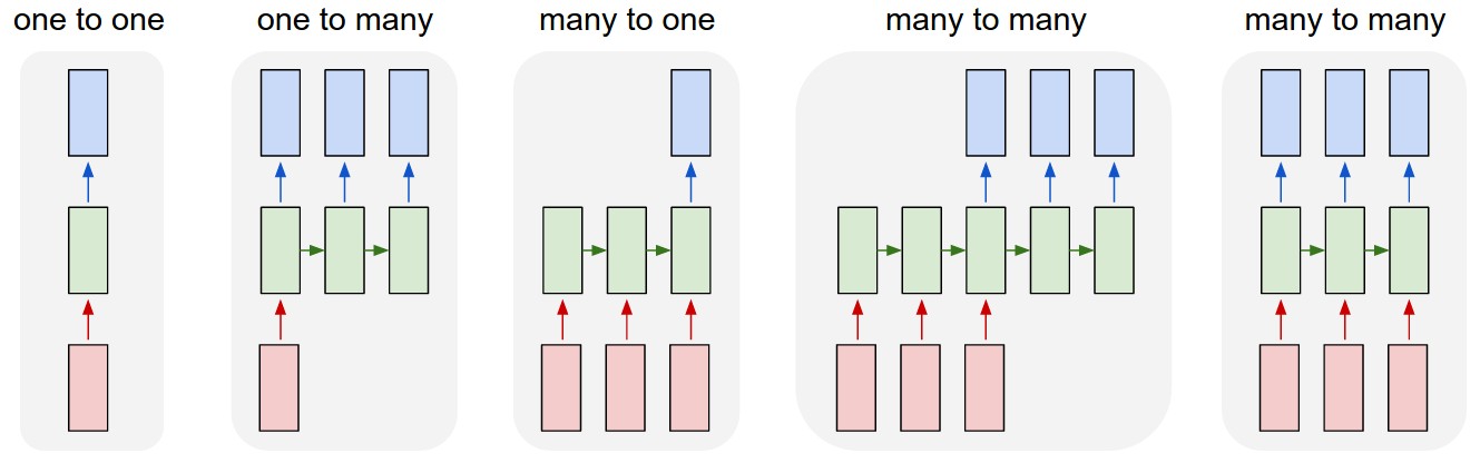
• one to one: image classification
• one to many: image captioning
• many to one: sentiment analysis
• many to many: machine translation
• many to many: video understanding

[From A. Karpathy Blog]

Example 1

• Multiple object recognition with visual attention, Ba et al.

Example 2

• DRAW: a recurrent neural network for image generation, Gregor et al.

$\newcommand{\bx}{\mathbf{x}}$

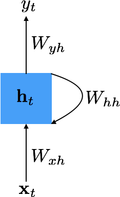
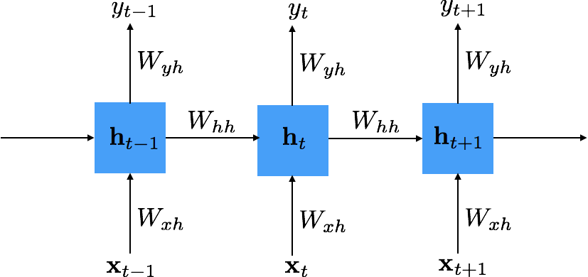
Recurrent Neural Network

• $\bh_t = \phi_1 \left( \bh_{t-1}, \bx_t \right)$
• $\hat{y}_t = \phi_2 \left( \bh_t \right)$

Where

• $\bx_t$ = input at time $t$
• $\hat{y}_t$ = prediction at time $t$
• $\bh_t$ = new state
• $\bh_{t-1}$ = previous state
• $\phi_1$ and $\phi_2$ = functions with parameters $W$s that we want to train

Subscript $t$ indicates sequence index.

Example

$$ \begin{split} \bh_t &= \tanh \left( W_{hh} \bh_{t-1} + W_{xh} \bx_t \right) \\ \hat{y}_t &= \text{softmax} \left( W_{hy} \bh_t \right) \end{split} $$

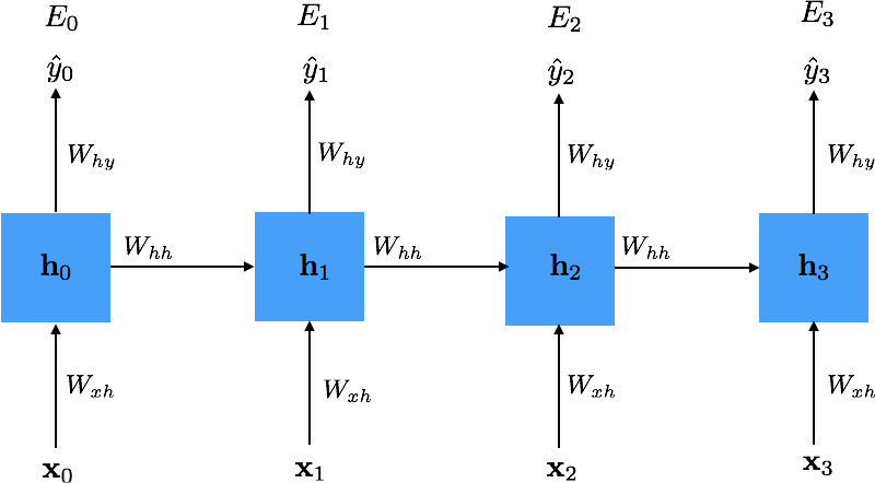
Unrolling in Time

• Parameters $W_{xh}$, $W_{hh}$ and $W_{hy}$ are tied over time
• Cost: $E = \sum_t E_t$, where $E_t$ depends upon $y_t$
• Training: minimize $E$ to estimate $W_{xh}$, $W_{hh}$ and $W_{hy}$

Loss

When dealing with output sequences, we can define loss to be a function of the predicted output $\hat{y}_t$ and the expected value $y_t$ over a range of times $t$

$$ E(y,\hat{y}) = \sum_t E_t(y, \hat{y}) $$

Example: using cross-entropy for k-class classification problem

$$ E(y,\hat{y}) = - \sum_t y_t \log \hat{y}_t $$

Computing Gradients

We need to compute $\frac{\partial E}{\partial W_{xh}}$, $\frac{\partial E}{\partial W_{hh}}$ and $\frac{\partial E}{\partial W_{hy}}$ in order to train an RNN

Example

$$ \frac{\partial E_3}{\partial W_{hh}} = \sum_{k=0}^3 \frac{\partial E_3}{\partial \hat{y}_3} \frac{\partial \hat{y}_3}{\partial \bh_3} \frac{\partial \bh_3}{\partial \bh_k} \frac{\partial \bh_k}{\partial W_{hh}} $$

Vanishing and Exploding Gradients

We can compute the highlighted term in the following expression using chain-rule $$ \frac{\partial E_3}{\partial W_{hh}} = \sum_{k=0}^3 \frac{\partial E_3}{\partial \hat{y}_3} \frac{\partial \hat{y}_3}{\partial \bh_3} \color{red}{\frac{\partial \bh_3}{\partial \bh_k}} \frac{\partial \bh_k}{\partial W_{hh}} $$ Applying the chain-rule $$ \frac{\partial \bh_3}{\partial \bh_k} = \prod_{j=k+1}^3 \frac{\partial \bh_j}{\partial \bh_{j-1}} $$ Or more generally $$ \frac{\partial \bh_t}{\partial \bh_k} = \prod_{j=k+1}^t \frac{\partial \bh_j}{\partial \bh_{j-1}} $$

Difficulties in Training

$$ \frac{\partial E_t}{\partial W_{hh}} = \sum_{k=0}^t \frac{\partial E_t}{\partial \hat{y}_t} \frac{\partial \hat{y}_t}{\partial \bh_t} \left( \prod_{j=k+1}^t \frac{\partial \bh_j}{\partial \bh_{j-1}} \right) \frac{\partial \bh_k}{\partial W_{hh}} $$

$\frac{\partial \bh_i}{\partial \bh_{i-1}}$ is a Jacobian matrix.

For longer sequences

• if $\left| \frac{\partial \bh_i}{\partial \bh_{i-1}} \right| < 0$, the gradients vanish
  • Gradient contributions from "far away" steps become zero, and the state at those steps doesn’t contribute to what you are learning.
  • Long short-term memory units are designed to address this issue
• if $\left| \frac{\partial \bh_i}{\partial \bh_{i-1}} \right| > 0$, the gradients explode
  • Clip gradients at a predefined threshold
• See also, On the difficulty of training recurrent neural networks, Pascanu et al.

Image Captioning Example

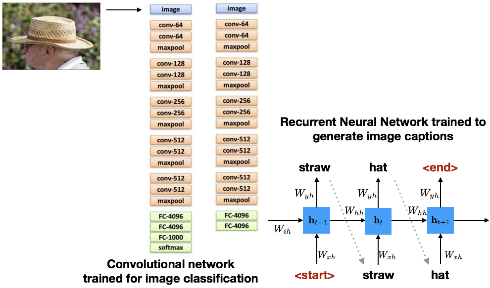
For the image captioning example shown in the previous slide, $\bh_t$ is defined as follows:

$$ \begin{split} \bh_t &= \tanh (W_{hh} \bh_{t-1} + W_{xh} \bx + \color{red}{W_{ih} \mathbf{v}}) \\ \hat{y}_t &= \text{softmax} (W_{hy} \bh_{t}) \end{split} $$

Image Captioning

• Explain Images with Multimodal Recurrent Neural Networks, Mao et al.
• Deep Visual-Semantic Alignments for Generating Image Descriptions, Karpathy - and Fei-Fei
• Show and Tell: A Neural Image Caption Generator, Vinyals et al.
• Long-term Recurrent Convolutional Networks for Visual Recognition and Description, Donahue et al.
• Learning a Recurrent Visual Representation for Image Caption Generation, Chen and Zitnick

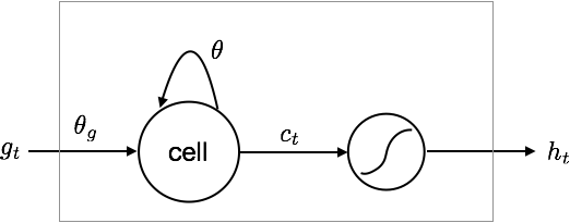
Dealing with Vanishing Gradients

Change of notation.

$$ \begin{split} c_t &= \theta c_{t-1} + \theta_g g_t \\ h_t &= \tanh(c_t) \end{split} $$

Long Short Term Memory (LSTM)

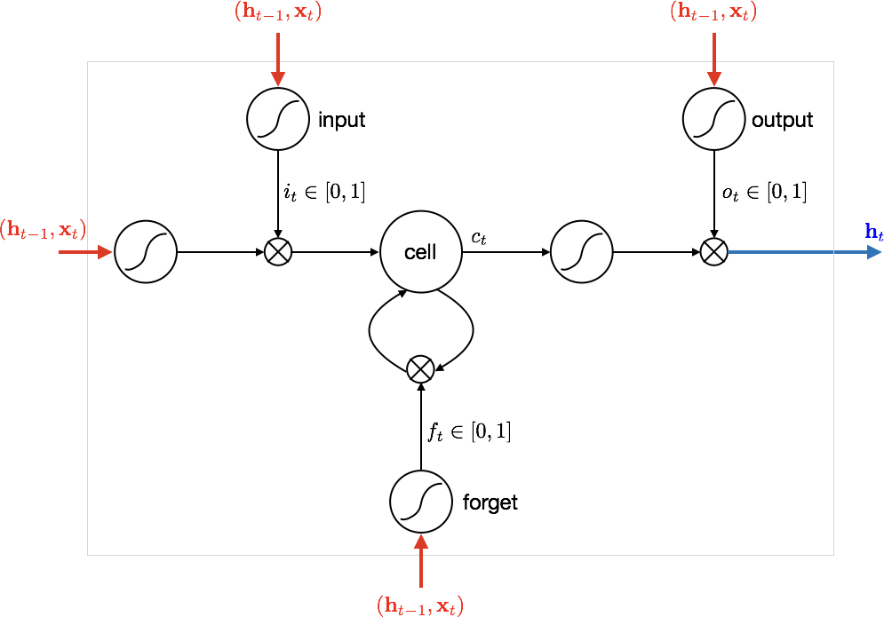
$\newcommand{\bi}{\mathbf{i}}$ $\newcommand{\bb}{\mathbf{b}}$ $\newcommand{\bc}{\mathbf{c}}$ $\newcommand{\bo}{\mathbf{o}}$ $\newcommand{\bo}{\mathbf{o}}$ $\newcommand{\bx}{\mathbf{x}}$ $\newcommand{\boldf}{\mathbf{f}}$

• Input gate: scales input to cell (write operation)
• Output gate: scales input from cell (read operation)
• Forget gate: scales old cell values (forget operation)

$$ \begin{split} \bi_t &= \text{sigmmoid}(\theta_{xi} \bx_t + \theta_{hi} \bh_{t-1} + \bb_{i}) \\ \boldf_t &= \text{sigmmoid}(\theta_{xf} \bx_t + \theta_{hf} \bh_{t-1} + \bb_{f}) \\ \bo_t &= \text{sigmmoid}(\theta_{xo} \bx_t + \theta_{ho} \bh_{t-1} + \bb_{o}) \\ \bg_t &= \tanh(\theta_{xg} \bx_t + \theta_{hg} \bh_{t-1} + \bb_{g}) \\ \bc_t &= \boldf_t \circ \bc_{t-1} + \bi_t \circ \bg_t \\ \bh_t &= \bo_t \circ \tanh(\bc_t) \end{split} $$

$\circ$ represent element-wise multiplication

RNN vs. LSTM

Check out the video at https://imgur.com/gallery/vaNahKE

Summary

• RNN
  • Allow a lot of flexibility in architecture design
  • Very difficult to train in practice due to vanishing and exploding gradients
  • Control gradient explosion via clipping
  • Control vanishing gradients via LSTMs
• LSTM
  • A powerful architecture for dealing with sequences (input/output)
  • Works rather well in practice