Gradient Descent
Faisal Qureshi
faisal.qureshi@ontariotechu.ca
http://www.vclab.ca
Lesson Plan
- Minimizing loss and the need for numerical techniques
- Gredient desent
- Recipe
- Update rule
- Batch update
- Mini-batch update
- Stochastic (or online) gradient descent
- Learning rate
- Changing learning rate to achieve faster convergence
- Newton's method
- How to choose a step size?
- Momentum
Regression
Consider data points $(x^{(1)}, y^{(1)}), (x^{(2)}, y^{(2)}), \cdots , (x^{(N)}, y^{(N)})$. Our goal is to learn a function $f(x)$ that returns (predict) the value $y$ given an $x$.
Linear regression
We assume that a linear model of the form $y=f(x)=\theta_0 + \theta_1 x$ best describe our data.
How do we determine the degree of "fit" of our model?
Least squares error
Loss/cost/objective function measures the degree of fit of a model to a given data.
A simple loss function is to sum the squared differences between the actual values $y^{(i)}$ and the predicted values $f(x^{(i)})$. This is called the least squares error.
$$ C(\theta_0, \theta_1) = \sum_{i=1}^N \left(y^{(i)} - f(x^{(i)}) \right)^2 $$
Our task is to find values for $\theta_0$ and $\theta_1$ (model parameters) to minimize the cost.
We often refer to the predicted value as $\hat{y}$. Specifically, $\hat{y}^{(i)} = f(x^{(i)})$.
$\DeclareMathOperator*{\argmin}{arg\,min}$
Minimizing cost
$$(\theta_0,\theta_1) = \argmin_{(\theta_0,\theta_1)} \sum_{i=1}^N \left(y^{(i)} - f(x^{(i)}) \right)^2$$
This is a convex function. We can solve for $\theta_0$ and $\theta_1$ by setting $\frac{\partial C}{\partial \theta_0}=0$ and $\frac{\partial C}{\partial \theta_1}=0$.
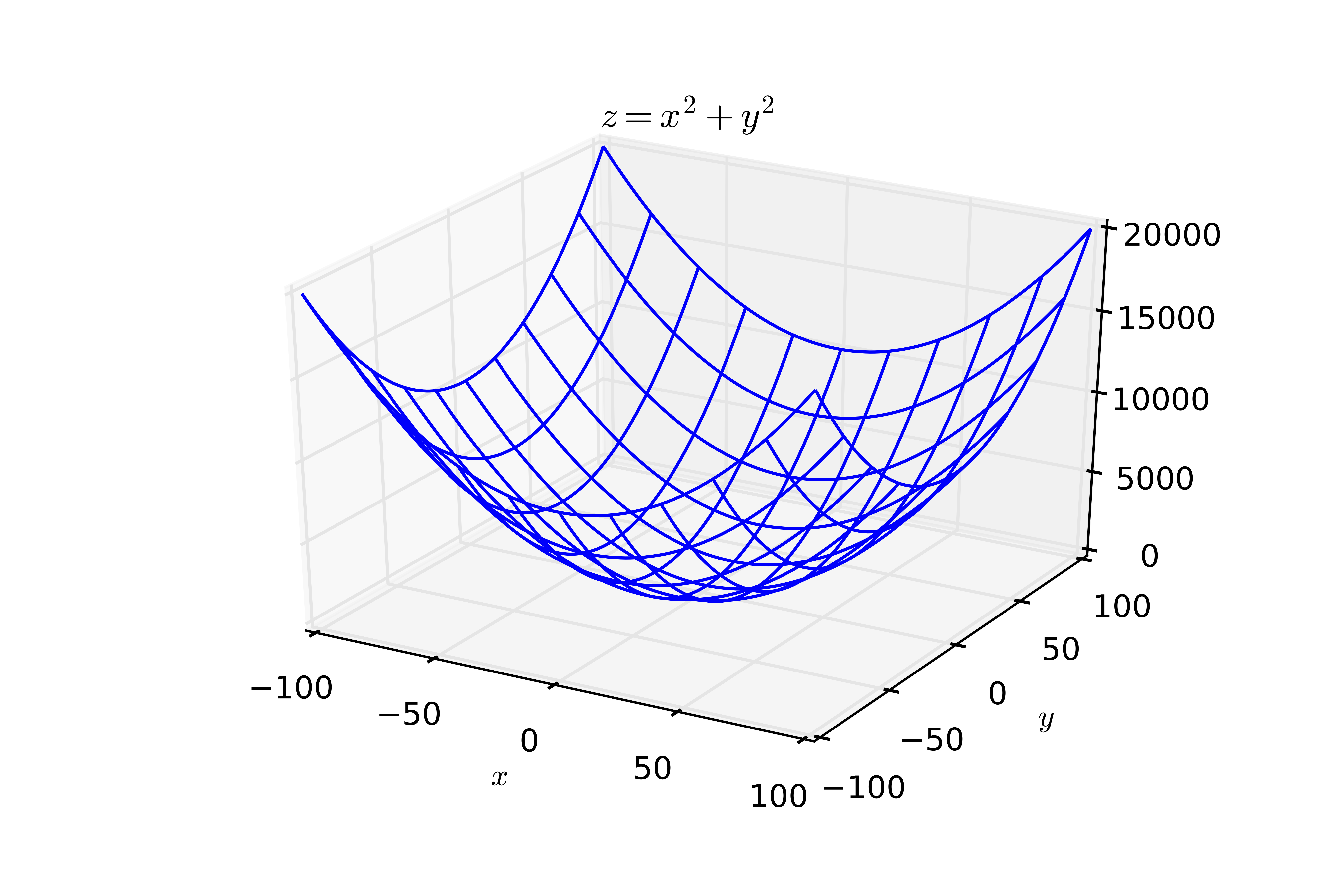
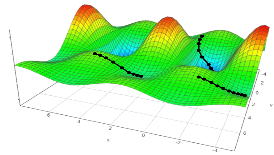
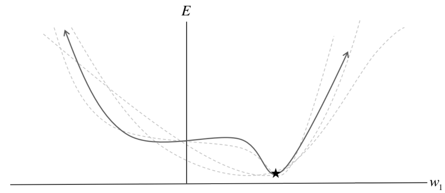
The need for numerical techniques
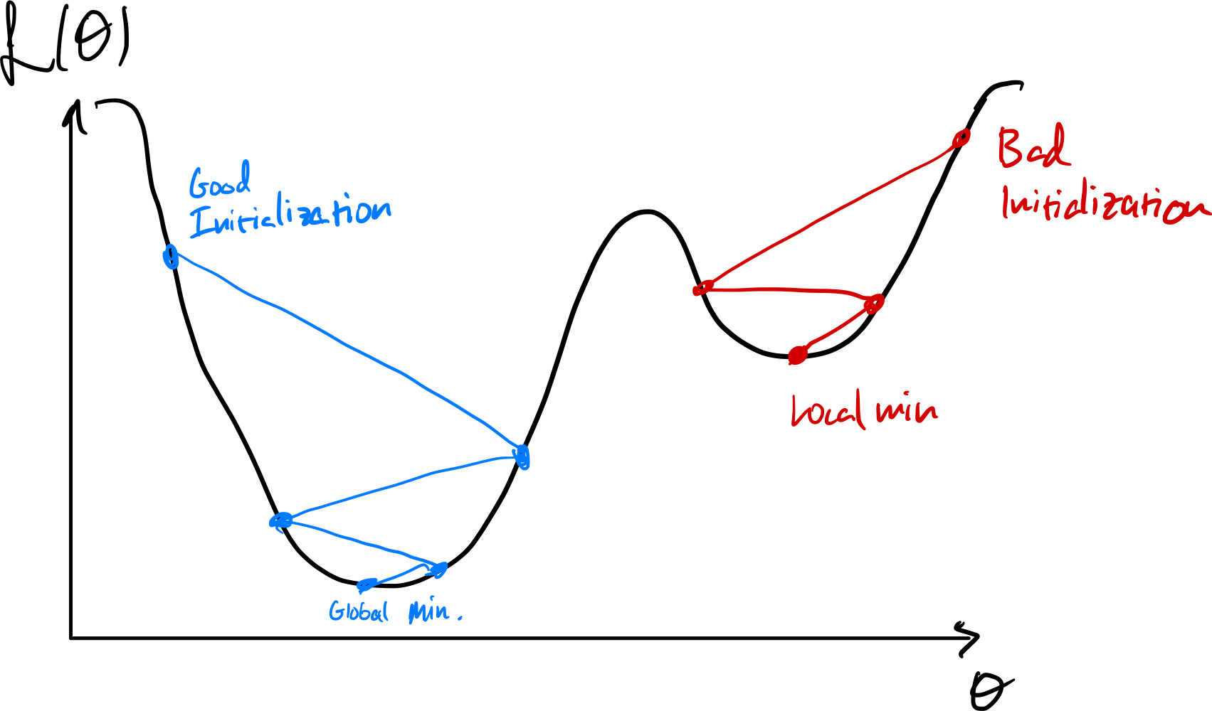
In general cost functions are not convex and it is not possible to find a minima (there are absolutely no guarantees about finding the global minima) using analytical methods
Gradient descent
A very powerful method of training the model parameters by minimizing the loss function. One of the simplest optimization methods. It is also referred to as steepest descent.
Recipe
- Initialize model parameters randomly (in our case $\theta$)
- Compute gradient of the loss function
- Take a step in the direction of negative gradient (decreasing loss function), and update parameters
- Repeat steps 2 to 4 until cannot decrease loss function anymore
Gradient
Let $\theta \in \mathbb{R}^D$ and $f(\theta)$ is a scalar-valued function. The gradient of $f(.)$ with respect to $\theta$ is:
$$ \nabla_{\theta} f(\theta) = \left[ \begin{array}{c} \frac{\partial f(\theta)}{\partial \theta_1} \\ \frac{\partial f(\theta)}{\partial \theta_2} \\ \frac{\partial f(\theta)}{\partial \theta_3} \\ \vdots \\ \frac{\partial f(\theta)}{\partial \theta_D} \end{array} \right] \in \mathbb{R}^D $$
Update rule
Gradient descent update rule is:
\begin{equation} \begin{split} \theta^{(k+1)} & = \theta^{(k)} - \eta \frac{\partial C}{\partial \theta} \\ & = \theta^{(k)} - \eta \nabla_{\theta} C \end{split} \end{equation}
$\eta$ is referred to as the learning rate. It controls the size of the step taken at each iteration.
Example: linear least squares fitting
For our 1D line fitting example, gradient descent update rule is $$\theta_0^{(k+1)} = \theta_0^{(k)} - \eta \frac{\partial C}{\partial \theta_0}$$ and $$\theta_1^{(k+1)} = \theta_1^{(k)} - \eta \frac{\partial C}{\partial \theta_1}$$
Where $$ \frac{\partial C}{\partial \theta_0} = -2 \sum_{i=1}^N \left(y^{(i)} - f(x^{(i)}) \right) \mathrm{ \ and\ } \frac{\partial C}{\partial \theta_1} = -2 \sum_{i=1}^N x^{(i)} \left(y^{(i)} - f(x^{(i)}) \right) $$
Fit
Batch update
- Sum or average updates across every example, then change the parameter values
Example
\begin{align} \theta_0^{(k+1)} &= \theta_0^{(k)} + 2 \sum_{i=1}^N \left(y^{(i)} - f(x^{(i)}) \right) \\ \theta_1^{(k+1)} &= \theta_1^{(k)} + 2 \sum_{i=1}^N x^{(i)} \left(y^{(i)} - f(x^{(i)}) \right) \end{align}
Mini-batch update
- Sum or average updates across a subset of the examples, then change the parameter values
- Examples in each batch are selected at random
Example
\begin{align} \theta_0^{(k+1)} &= \theta_0^{(k)} + 2 \sum_{i=1}^{N_{\mathrm{batch}}} \left(y^{(i)} - f(x^{(i)}) \right) \\ \theta_1^{(k+1)} &= \theta_1^{(k)} + 2 \sum_{i=1}^{N_{\mathrm{batch}}} x^{(i)} \left(y^{(i)} - f(x^{(i)}) \right) \end{align}
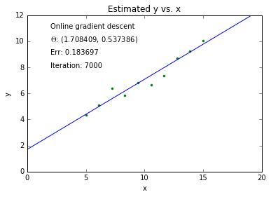
Stochastic or online gradient desent
- Update parameter values for each training example in turn
- This assumes that sample is i.i.d. (independent, identically distributed)
- This is particularly useful when dealing with very large datasets
Example
\begin{align} \theta_0^{(k+1)} &= \theta_0^{(k)} + 2 \left(y^{(i)} - f(x^{(i)}) \right) \\ \theta_1^{(k+1)} &= \theta_1^{(k)} + 2 x^{(i)} \left(y^{(i)} - f(x^{(i)}) \right) \end{align}
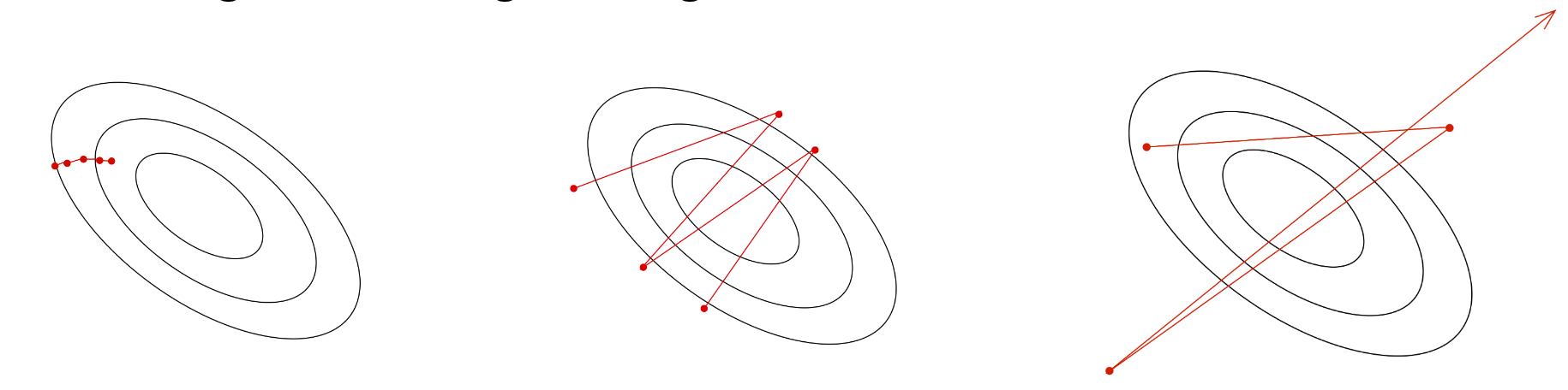
The effects of using a subset of data to compute loss
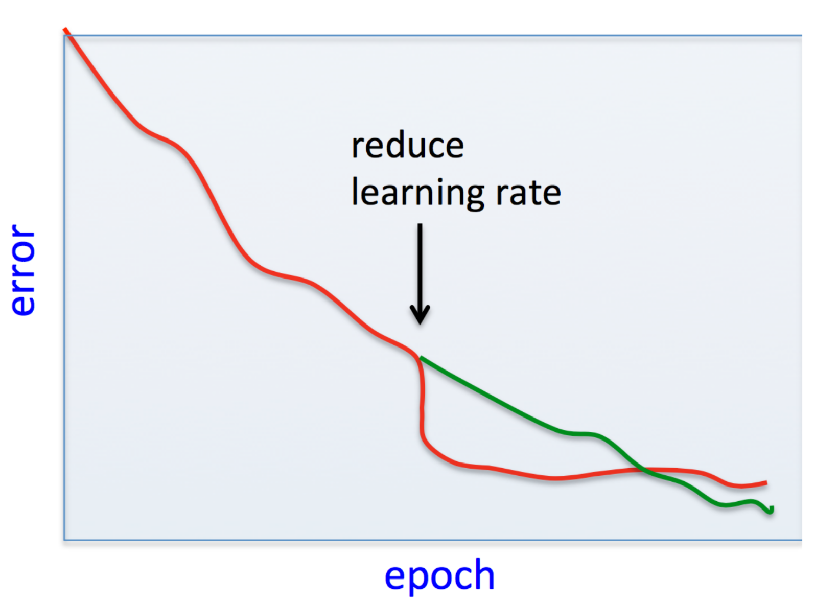
Learning rate
$$ \theta^{(k+1)} = \theta^{(k)} - \eta \nabla_{ \theta}{C} $$
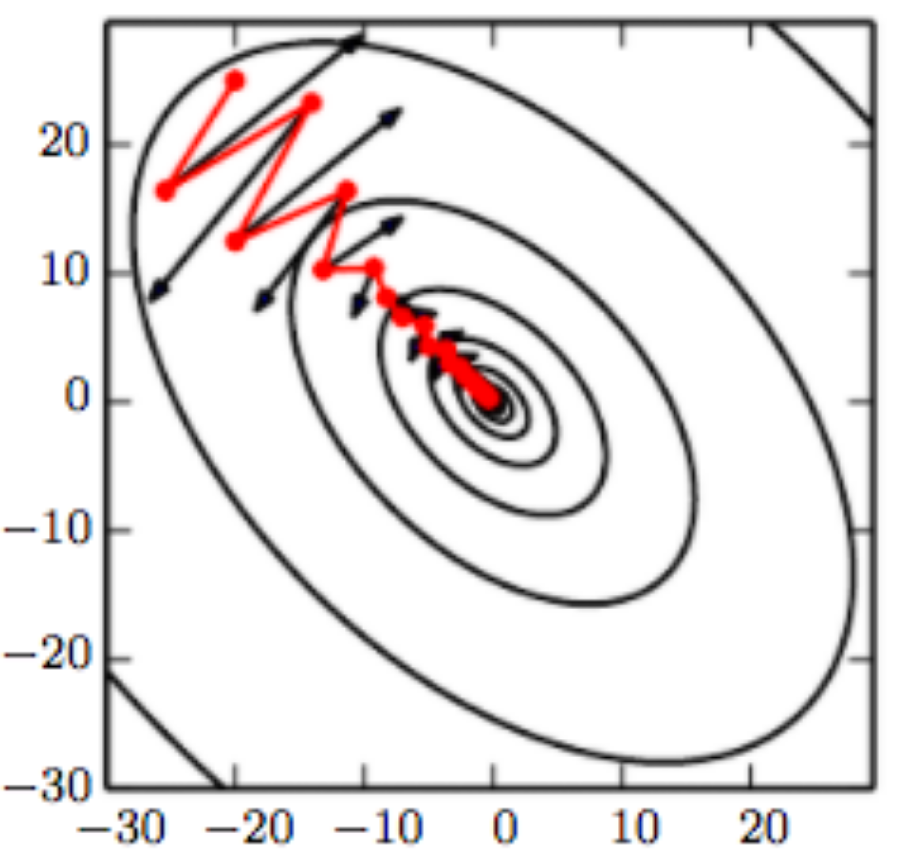
- $\eta$ too large, and the system might not converge
- $\eta$ too small, and the system might take too long to converge
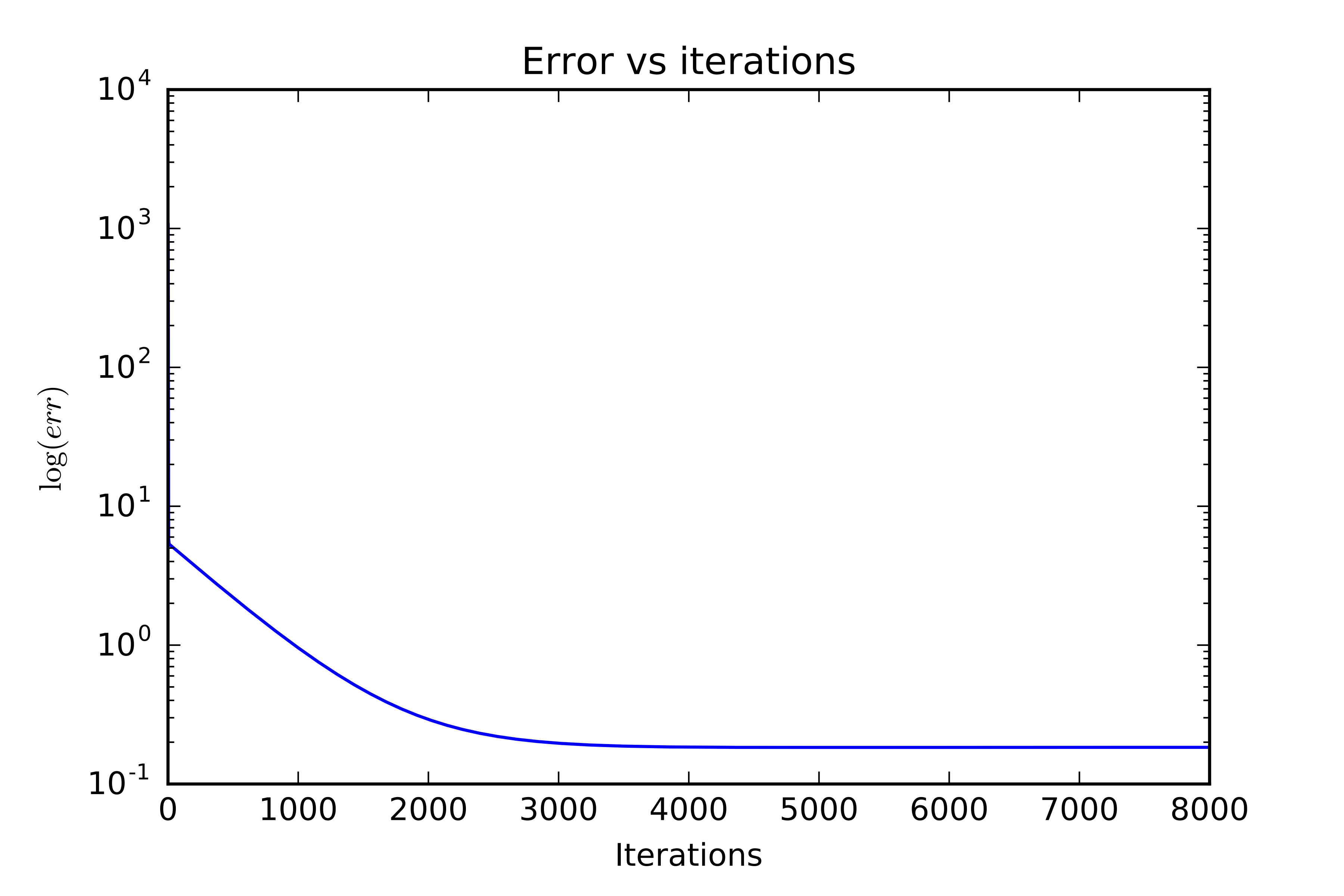
For gradient descent, $C(\theta)$, i.e., the objective, should decrease after every step.
A common scheme is stop iterations (i.e., declare convergence) if decrease in $C(\theta)$ is less than some threshold $\epsilon$ (say $10^{-3}$) in one iteration.
General rule of thumb: If gradient descent isn't working, use a smaller $\eta$.
Too small or too large a learning rate
Newton's method
We have looked at gradient descent, now we look at another method that can be used to estimate parameters $\theta$'s. This method converges much faster than gradient descent.
Problem: Given $f(\theta)$, find $\theta$ s.t. $f(\theta) = 0$
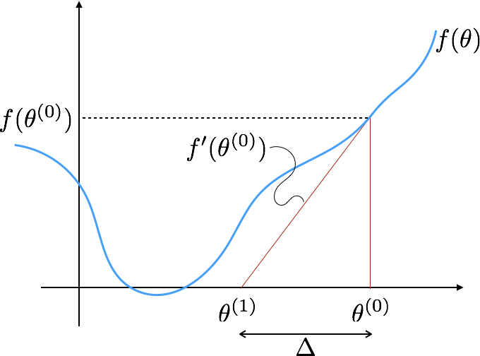
Observation
Gradient is the slope of the function.
$$ \begin{split} f'(\theta^{(0)}) &= \frac{f(\theta^{(0)})}{\Delta} \\ &= \frac{f(\theta^{(0)})}{\theta^{(1)} - \theta^{{0}}} \end{split} $$
Method
An iterative method to solve the above problem is:
- Start with an initial value of $\theta$
- Update $\theta$ as follows $$ \theta^{(1)} = \theta^{(0)} - \frac{f(\theta^{(0)})}{f'(\theta^{(0)})} $$
- Repeat until $f(\theta) \approx 0$ or maximum number of iterations have reached.
Using Newton's method to maximize (or minimize a function)
We are interested in maximizing or minimize a function, e.g., we minimize the negative log likelihood to estimate the parameters.
Gradient is $0$ at maxima, minima and saddle points of a function. We can use the following update rule to maximize or minimize a function.
$$ \theta^{(1)} = \theta^{(0)} - \frac{C'(\theta^{(0)})}{C''(\theta^{(0)})} $$
Hessian
The Hessian matrix of $f(.)$ w.r.t. $\theta$, written $\nabla_{\theta}^2 f(\theta)$ or simply $\mathbf{H}$, is a $d \times d$ matrix of partial derviatives.
\begin{equation*} \mathbf{H} = \left[ \begin{array}{cccc} \frac{\partial^2 f(\theta)}{\partial \theta^2} & \frac{\partial^2 f(\theta)}{\partial \theta_1 \partial \theta_2} & \cdots & \frac{\partial^2 f(\theta)}{\partial \theta_1 \partial \theta_D} \\ \frac{\partial^2 f(\theta)}{\partial \theta_2 \theta_1} & \frac{\partial^2 f(\theta)}{\partial \theta_2^2} & \cdots & \frac{\partial^2 f(\theta)}{\partial \theta_2 \partial \theta_D} \\ \vdots & \vdots & & \vdots \\ \frac{\partial^2 f(\theta)}{\partial \theta_D \theta_1} & \frac{\partial^2 f(\theta)}{\partial \theta_D \partial \theta_2} & \cdots & \frac{\partial^2 f(\theta)}{\partial \theta_D^2} \\ \end{array} \right] \end{equation*}
How to choose the step size?
The most basic second-order optimization algorithm is Newton's algorithm.
$$ \theta^{(k+1)} = \theta^{(k)} - \mathbf{H}_{k}^{-1} \mathbf{g}_k $$
$\mathbf{H}_{k}$ is Hessian at step $k$
$\mathbf{g}_k$ gradient at step $k$
Momentum
$$\Delta \theta^{(k+1)} = \alpha \Delta \theta^{(k)} + (1 - \alpha) (- \eta) (\nabla C(\theta))$$
Why momentum really works (interactive)
Summary
- Gradient descent
- Batch update
- Online or stochastic
- Learning rate
- Momentum
- Hessian
- These methods work well in practice
- All of these methods converge as long as the learning rate is sufficiently small
- The speed of convergence differs great, however
- Newton's method converges quadratically
- Every iteration of Newton's method doubles the number of digits to which your solution is accurate, e.g., error goes from 0.01 to 0.0001 in one step
- This only holds when already close to the solution
- $\theta$ is initialized randomly