Autoencoders
Faisal Qureshi
faisal.qureshi@ontariotechu.ca
http://www.vclab.ca
Credits
These notes draw heavily upon the excellent machine learning lectures put together by Roger Gross and Jimmy Ba.
Lesson Plan
- Autoencoders
- Variational autoencoders
- Class-conditional autoencoders
Goal
- Learn representations of images, text, sound, etc. in an unsupervised manner
Autoencoder
- An autoencoder is a feedforward network
- Input: $\mathbf{x}$
- Output: $\mathbf{x}$
- To make this problem non-trivial, we force the input to pass through a bottleneck layer
- Dimension of the bottleneck layer is much smaller than the input layer
Putting it all together
Encoder network constructs the latent representation $\mathbf{z}$:
$$ \mathbf{z} = \mathcal{E}(\mathbf{x}; \theta_e) $$
and decoder network reconstructs $\mathbf{x}$ given it's latent representation:
$$ \mathbf{x} = \mathcal{D}(\mathbf{z}; \theta_d). $$
Encoder $\mathcal{E}$ and decoder $\mathcal{D}$ are paramterized by $\theta_e$ and $\theta_d$, respectively.
Training an autoencoder
Parameters of the encoder and decoder are updated using a single pass of the ordinary backprop. Since this goal is signal reconstruction, it is common to minimize the reconstruction loss when training an autoencoder
$$ \mathcal{L}_{\text{AE}}(\mathbf{x}; \theta) = \| \mathbf{x} - \mathbf{\hat{x}} \|^2, $$where $\mathbf{x}$ is the input, $\mathbf{\hat{x}}$ is its reconstruction, and $\theta = (\theta_e, \theta_d)$.
Uses of autoencoders
- Most obvious use is compression (i.e., reducing the size of the data)
- Map high-dimensional data to 2D or 3D for visualization
- Learn features or representations in an unsupervised manner
- These representations can be subsequently used in supervised tasks
- Perhaps learn semantically meaningful relationships
Non-linear dimensionality reduction
- Autoencoders perform a kind of non-linear dimensionality reduction
- These project data, not onto a subspace (as in Principle Component Analysis (PCA)), but onto a non-linear manifold
- Autoencoders are able to learn more powerful codes than, linear methods, say PCA, for a given dimensionality
Limitations
- Autoencoders are not generative models
- It is not possible to generate new examples from a given autoencoder
- Because the latent space does not define a probability distribution, it is not possible to sample from this distribution and use the decoder section to generate a new data sample
- Why do we care?
- It is not possible to generate new examples from a given autoencoder
- How do we choose a "good" latent dimension?
Variational Autoencoder
Observation model
Consider that the latent space defines a probability distribution $p(\mathbf{z})$. We can then sample $\mathbf{z}$ from this distribution. Given $\mathbf{z}$, we can use the decoder to generate $\mathbf{x}$:
$$ p(\mathbf{x}) = \int p(\mathbf{x | z}) p(\mathbf{z}) d \mathbf{z}. $$
Recall that decoder is deterministic. When $\mathbf{z}$ is low-dimensional, $p(\mathbf{x}) = 0$ almost everywhere. The model generates data samples that lie on a low-dimensional sub-manifold of $\mathcal{X}$. This reduces data samples diversity.
This can be fixed by using a noisy observation model:
$$ p(\mathbf{x | z}) = \mathcal{N} \left( \mathbf{x}; G_\theta(\mathbf{z}), \eta \mathbf{I} \right), $$
where $G_\theta(\mathbf{z})$ denotes decoder (or generator) parameterized by $\theta$.
The decoder function $G_\theta{\mathbf{z}}$ is very complicated and there is no hope of finding a closed-form solution to the integral shown above.
Solution: Instead let's maximize the lower-bound on $\log p(\mathbf{x})$. In lieu of maximizing $\log p(\mathbf{x})$, which would require us to compute the integral.
Variational inference
Jensen's Inequality: for a convex function $h$ of a random variable $X$
$$ \mathtt{E}[h(X)] \ge h(\mathtt{E}[X]). $$
It follows that if $h$ is concave (i.e., $-h$ is convex)
$$ \mathtt{E}[h(X)] \le h(\mathtt{E}[X]). $$
Note that $\log z$ is concave; therefore,
$$ \mathtt{E}[\log X] \le \log \mathtt{E}[X]. $$
We will use Jensen's Inequality to define the lower-bound. We have
$$ p(\mathbf{x}) = \int p(\mathbf{x | z}) p(\mathbf{z}) d \mathbf{z}. $$
Taking $\log$ of both sides and assuming we have some distribution $q(\mathbf{z})$. (For the moment, don't worry about this distribution.)
$$ \begin{align} \log p(\mathbf{x}) &= \log \int p(\mathbf{x | z}) p(\mathbf{z}) d \mathbf{z} \\ &= \log \int \frac{q(\mathbf{z})}{q(\mathbf{z})} p(\mathbf{x | z}) p(\mathbf{z}) d \mathbf{z} \\ &= \log \int q(\mathbf{z}) \frac{p(\mathbf{z})}{q(\mathbf{z})} p(\mathbf{x | z}) d \mathbf{z} \\ &\ge \int q(\mathbf{z}) \log \left[ \frac{p(\mathbf{z})}{q(\mathbf{z})} p(\mathbf{x | z}) \right] d \mathbf{z} \hspace{1cm} \text{(Jenson's Inequality)} \\ &= \mathtt{E}_q \left[ \log \frac{p(\mathbf{z})}{q(\mathbf{z})} \right] + \mathtt{E}_q \left[ \log p(\mathbf{x} | \mathbf{z}) \right] \end{align} $$
This
$$ \mathtt{E}_q \left[ \log \frac{p(\mathbf{z})}{q(\mathbf{z})} \right] + \mathtt{E}_q \left[ \log p(\mathbf{x} | \mathbf{z}) \right] $$
is the lower-bound of $\log p(\mathbf{x})$.
Kullback-Leibler (KL) divergence
KL divergence, a commonly-used measure of "distance" between two probability distributions, is defined as
$$ D_{KL} \left( q(\mathbf{z}) || p(\mathbf{z}) \right) = \mathtt{E}_q \left[ \log \frac{q(\mathbf{z})}{p(\mathbf{z})} \right]. $$
So, term
$$ \mathtt{E}_q \left[ \log \frac{p(\mathbf{z})}{q(\mathbf{z})} \right] $$
is just negative KL-divergence.
We often desire $p(\mathbf{z}) = \mathcal{N}(\mathbf{0}, \mathbf{I})$, so the KL-term encourages $q$ to be close to $\mathcal{N}(\mathbf{0}, \mathbf{I})$.
Reconstruction error
Recall our observation model, which is
$$ p(\mathbf{x | z}) = \mathcal{N} \left( \mathbf{x}; G_\theta(\mathbf{z}), \eta \mathbf{I} \right). $$
It follows
$$ \begin{align} \log p(\mathbf{x | z}) &= \log \mathcal{N} \left( \mathbf{x}; G_\theta(\mathbf{z}), \eta \mathbf{I} \right) \\ &= \log \left[ \frac{1}{(2 \pi \eta)^{D/2}} \right] \exp \left( - \frac{1}{2 \eta} \| \mathbf{x} - G_\theta(\mathbf{z}) \|^2 \right) \\ &= - \frac{1}{2 \eta} \| \mathbf{x} - G_\theta(\mathbf{z}) \|^2 + \text{const} \end{align} $$
This is simply the reconstruction error.
Variational inference
We are minimizing the variational lower bound or variational free energy
$$ \log p (\mathbf{x}) \ge \mathcal{F}(\theta, q) = - D_{KL}(q || p) + \mathtt{E}_q \left[ \log p(\mathbf{x} | \mathbf{z}) \right] $$
We need to pick $q$ to make the bound as tight as possible. This is achieved by selecting $q$ as close to the posterior distribution $p( \mathbf{z} | \mathbf{x} )$ (note this is the probabilistic view of the encoder stage of the autoencoder).
The reconstruction term is minimized when $q$ is a point mass
$$ \DeclareMathOperator*{\argmin}{arg\,min} \mathbf{z}_* = \argmin_{\mathbf{z}} \| \mathbf{x} - G_\theta(\mathbf{z}) \|^2, $$
however point masses have infinite KL-divergence. Therefore, the KL-divergence term forces $q$ to spread out.
Reparameterization trick
Let's turn our attention to $q$. To keep things simple, let's assume that $q$ is a Gaussian distribution. (Recall that the KL-divergence term will force $p(\mathbf{z})$ to be as close to $q$ as possible.)
Specifically,
$$ q(\mathbf{z}) = \mathcal{N}( \mathbf{z} ; \mathbf{\mu}, \Sigma ), $$
where
$$ \mathbf{\mu} = \left( \mu_1, \mu_2, \cdots, \mu_K \right) $$
and
$$ \Sigma = \mathrm{diag} \left( \sigma_1^2, \sigma^2_2, \cdots, \sigma_K^2 \right). $$
In general it is difficult to differentiate through an expectation, but since we have assign $q$ to be a Gaussian distribution, we can apply the reparameterization trick
$$ z_i = \mu_i + \sigma_i \epsilon_i, $$
where
$$ \epsilon_i \sim \mathcal{N}(0, 1). $$
Training a variational autoencoder
Idea 1
One way to maximize $\mathcal{F}(\theta, q)$ is to use Expectation-Maximization method:
- Fit $q$ to posterior distribution of $\mathbf{x}$ by doing many steps of gradient ascent on $\mathcal{F}$, and
- Update $\theta$, again with gradient ascent on $\mathcal{F}$.
This process requires many iterations for each training sample, and it is expensive.
Idea 2
Learn an inference network that predicts $(\mathbf{\mu}, \Sigma)$ as a function of $\mathbf{x}$. This inference network (we will soon see that this is simply an encoder) outputs $\mathbf{\mu}$ and $\log \sigma$. $\log \sigma$ ensures $\sigma > 0$. $\sigma \approx 0$ means that the inference network is deterministic (this will reduce this inference network to behave just like the encoder of an "ordinary" autoencoder). Aside: the KL-divergence term will forces $\sigma > 0$, so the latent representation $\mathbf{z}$ constructed by this inference network will be noisy.
We combine this with a decoder stage and note that the structure closely resembles an autoencoder. Hence the name, variational autoencoder.
The variational autoencoder can be trained just like an "ordinary" autoencoder. Encoder and decoder parameters are updated using a single pass of the ordinary backprop. The reconstruction term resembles the reconstruction error used to train "ordinary" autoencoders and the KL-divergence term acts as a regularizer and forces $\mathbf{z}$ to be more stochastic.
For VAE we minimize the following loss
$$ \mathcal{L}_{\text{VAE}}(\mathbf{x}; \theta, \phi) = - D_{KL}(q_\phi(\mathbf{z} | \mathbf{x}) || p_\theta( \mathbf{z} | \mathbf{x} ) ) + \mathtt{E}_q \left[ \log p_\theta(\mathbf{x} | \mathbf{z}) \right] $$VAEs vs. other generative models
- VAEs are "easy" to train, just like autoencoders (note that we have dropped the adjective "ordinary.")
- VAEs are able to generate new samples in a single pass, unlike autoregressive models
- VAEs are able to fit low-dimensional latent space, unlike reversible models
Class-conditional VAEs
Class-conditional VAEs provide labels to both encoder and decoder.
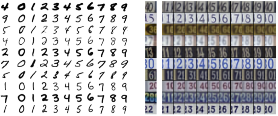
Consider a VAE for image reconstruction. Say we have class labels available for each image. E.g., we have a collection of cats and dogs images where each image consists of a cat or dog label. By providing these labels to the VAE, we free up the latent representation to learn "style" of the image (i.e., the visual appearance of cat or dog). It no longer has to learn the class of the image. Thus, a class-conditional VAE can potentially disentangle content from style. This opens up many interesting applications. Take care, however, since disentangling style from content is challenging and requires careful tuning.
Varying two latent dimensions (i.e., $\mathbf{z}) while holding $y$ fixed.

Varying the label $y$ fixed, while hold $\mathbf{z}$ fixed.

Loss for class-conditional VAEs
Loss for class-conditional VAEs is arrived at using a similar analysis to the loss for VAE. It is given below
$$ \mathcal{L}_{\text{CVAE}}(\mathbf{x}, \mathbf{y}; \theta, \phi) = - D_{KL}(q_\phi(\mathbf{z} | \mathbf{x}, \mathbf{y}) || p_\theta( \mathbf{z} | \mathbf{x} ) ) + \mathtt{E}_q \left[ \log p_\theta(\mathbf{y} | \mathbf{x}, \mathbf{z}) \right]. $$Here $\mathbf{y}$ denotes class labels.
Latent space interpolation
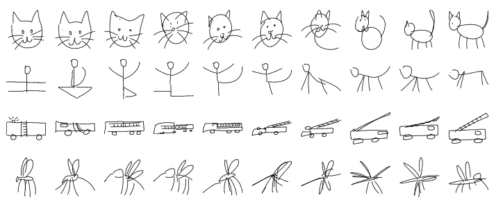
It is possible to generate interesting samples by interpolating between two vectors of the latent space.

References
- Reducing the Dimensionality of Data with Neural Networks, G.E. Hinton and R.S. Salakhutdinov, Science, 2006.
- Auto-Encoding Variational Bayes, D.P. Kingma and M. Walling, 2013.
- Learning Structured Output Representation using Deep Conditional Generative Models, K. Sohn, X. Yan, H. Lee, NeurIPS, 2015.
- A Neural Representation of Sketch Drawings, D. Ha, D. Eck, 2017.
