Neural Networks
Faisal Qureshi
http://www.vclab.ca
Lesson Plan
- Feed-forward neural networks
- Activation functions
- Gradient based learning in neural networks
- Backpropagation
- Layered view of neural networks
Feed forward neural networks
- Approximate some function $y=f^{*}(\mathbf{x})$ by learning parameters $\theta$ s.t. $\tilde{y} = f(\mathbf{x}; \theta)$
- Feed forward neural networks can be seen as directed acyclic graphs $$ y = f(\mathbf{x}) = f^{(3)}(f^{(2)}(f^{(1)}(\mathbf{x}))) $$
- Training examples specify the output of the last layer
- Network needs to figure out the inputs/outputs for the hidden layers
Extending linear models
How can we extend linear models?
- Specify a very general $\phi$ s.t. the model becomes $y=\theta^T \phi(\mathbf{x})$
- Problem with generalization
- Difficult to encode prior information needed to solve AI-level tasks
- Engineer $\phi$ for the task at hand
- Tedious
- Difficult to transfer to new tasks
- Neural networks approaches
- $y = f(\mathbf{x} ; \theta, w) = \phi(\mathbf{x}; \theta)^T w$ i.e. use parameters $\theta$ to learn $\phi$ and use $w$ to map $\phi(\mathbf{x})$ to the desired output $y$
- The training problem is non-convex
- Key advantage: a designer just need to specify the right family of functions and not the exact function $\phi$
Classical artificial neural networks
- Shallow and wide
- One hidden layer can represent any function
- Focus was on efficient ways to optimize (train)
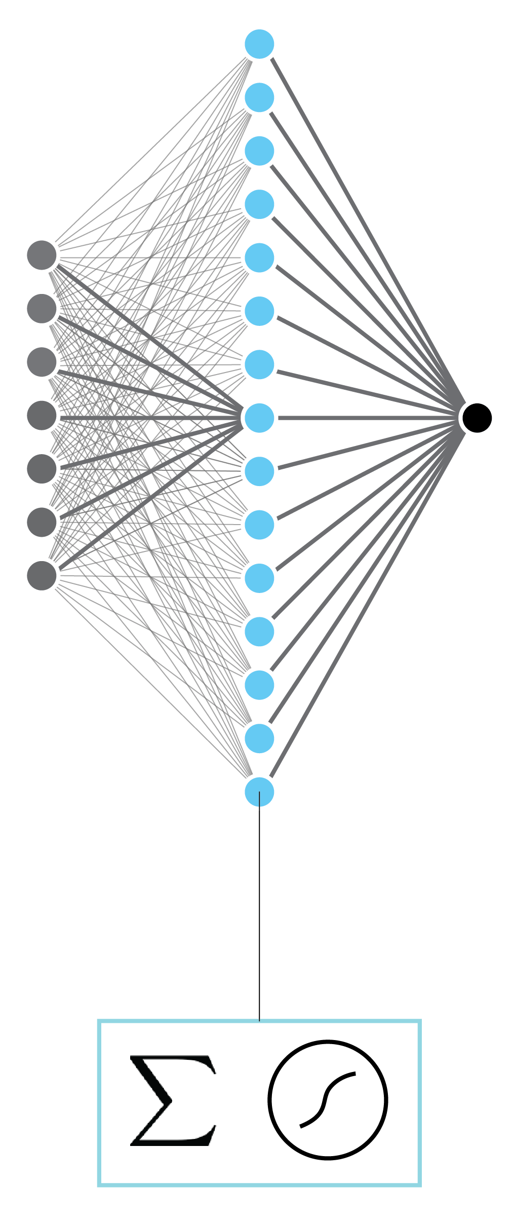
Mathematically
We can represent the above network as:
$$ y = f_o \left( \mathbf{W}_{oh} f_h \left( \mathbf{W}_{ih} \mathbf{x} \right) \right). $$
Here, $\mathbf{x} \in \mathbb{R}^d$ is the d-dimensional input, $\mathbf{W}_{ih} \in \mathbb{R}^{d_h \times d}$ is the input-to-hidden-layer weight matrix, $d_h$ is the size of the hidden layer, $\mathbf{W}_{ho} \in \mathbb{R}^{1 \times d_h}$ is the hidden-layer-to-output weight matrix, and $f_h$ and $f_o$ are activations functions for hidden layer and output, respectively. Activation functions take a vector as input and return a vector of the same size. The function is applied element-wise.
Traditionally, possible choices for $f_h$ are:
- hyperbolic tangent; and
- sigmoid.
Q. What if we use linear activation functions throughout?
Activation functions
import numpy as np
import matplotlib.pyplot as plt
def sigmoid(x):
  return 1 / (1 + np.exp(-x))

x = np.linspace(-5,5,100)

plt.figure(figsize=(10,5))
plt.suptitle('Activation functions')
plt.subplot(1,2,1)
plt.title('$tanh$')
plt.plot(x, np.tanh(x))
plt.xlabel('$x$')
plt.grid()
plt.subplot(1,2,2)
plt.title('$sigmoid$')
plt.xlabel('$x$')
plt.grid()
plt.plot(x, sigmoid(x));

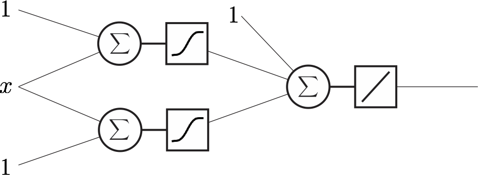
Example: a regression network
- Input: 1D, real numbers
- Ouput: 1D, real numbers
- Hidden layer size: 2
- Number of weights: 7
- Loss: MSE
- Statistics connection: line fitting
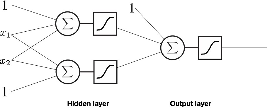
Example: a classification network
- Input: 2D, real numbers
- Output: 1D, class labels 0 or 1
- Hidden layer size: 2
- Number of weights: 9
- Loss: Cross-entropy
- Statistics connect: probabilitist view of line fitting
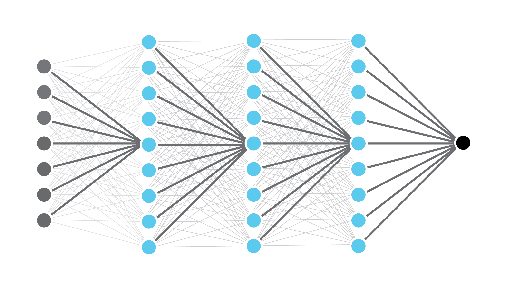
Deep neural networks
- Multi-layer networks
- These networks are deeper than these are wider
- Hierarchical representation
- Reduces semantic gap
- Deep networks outperform humans on many tasks
- Access to data
- Advances in computer science, physics and engineering
Activation functions
- The activation function for output:
- Identity function for regression;
- Sigmoid for binary classification; and
- Softmax for multi-class classification.
- The following activation functions are typically used for hidden layers.
import torch
import torch.nn as nn
x = torch.linspace(-10,10,100)

plt.figure(figsize=(20,10))
plt.subplot(2,4,1)
plt.title('ReLU')
plt.grid()
plt.plot(x.numpy(), nn.ReLU()(x).numpy())
plt.subplot(2,4,2)
plt.title('Leaky ReLU')
plt.grid()
plt.plot(x.numpy(), nn.LeakyReLU(0.1)(x).numpy())
plt.subplot(2,4,3)
plt.title('ELU')
plt.grid()
plt.plot(x.numpy(), nn.ELU()(x).numpy())
plt.subplot(2,4,4)
plt.title('Hardswish')
plt.grid()
plt.plot(x.numpy(), nn.Hardswish()(x).numpy())
plt.subplot(2,4,5)
plt.title('GeLU')
plt.grid()
plt.plot(x.numpy(), nn.GELU()(x).numpy())
plt.subplot(2,4,6)
plt.title('Mish')
plt.grid()
plt.plot(x.numpy(), nn.Mish()(x).numpy())
plt.subplot(2,4,7)
plt.title('CELU')
plt.grid()
plt.plot(x.numpy(), nn.CELU()(x).numpy())
plt.subplot(2,4,8)
plt.title('ReLU6')
plt.grid()
plt.plot(x.numpy(), nn.ReLU6()(x).numpy());

- Check PyTorch Documentation for a complete list of activation functions used in deep learning
Gradient-based learning in neural networks
- Non-linearities of neural networks render most cost functions non-convex
- Use iterative gradient based optimizers to drive cost function to lower values
- Gradient descent applied to non-convex cost functions provides no guarantees, and it is sensitive to initial conditions
- Initialize weights to small random values
- Initialize biases to zero or small positive values
Q. How to compute the gradient of cost w.r.t. to network parameters.
Computing gradients
- Backpropagation (Rumelhard et al. 1986) is often used to compute the gradient of the error function w.r.t. to network's weights.
- We will examine backpropagation within a layered view of neural networks
- Treating neural networks as differentiable layers allows a plug-and-play compositional ability enabling us to construct large neural networks
Example: Two-class softmax classifier
We can define the negative log likelihood for a two-class softmax classifier as
$$ \small \begin{split} l(\theta) = - \sum_{i=1}^N \mathbb{I}_0 (y^{(i)}) \log \frac{e^{\mathbf{x}^{(i)^T} \theta_1}}{e^{\mathbf{x}^{(i)^T} \theta_1} + {e^{\mathbf{x}^{(i)^T} \theta_2}}} + \mathbb{I}_1 (y^{(i)}) \log \frac{e^{\mathbf{x}^{(i)^T} \theta_2}}{e^{\mathbf{x}^{(i)^T} \theta_1} + {e^{\mathbf{x}^{(i)^T} \theta_2}}} \end{split}. $$
We use the negative log likelihood as the cost $C(\theta)$ for this problem. We need to compute the gradient of this loss w.r.t. network paramters for gradient-based learning.
We can represent this network as layers as follows.
Chain rule
$$ \frac{\partial f(g(u,v),h(u,v))}{\partial u} = \frac{\partial f}{\partial g} \frac{\partial g}{\partial u} + \frac{\partial f}{\partial h} \frac{\partial h}{\partial u} $$

We can use the chain rule to compute $\frac{\partial z^4}{\partial \theta_1}$ and $\frac{\partial z^4}{\partial \theta_2}$.
$$ \begin{eqnarray} \frac{\partial z^4}{\partial \theta_1} &=& \frac{\partial z^4}{\partial z_1^3} \frac{\partial z_1^3}{\partial \theta_1} + \frac{\partial z^4}{\partial z_2^3} \frac{\partial z_2^3}{\partial \theta_1} \\ &=& \frac{\partial z^4}{\partial z_1^3} \left( \frac{\partial z^3_1}{\partial z_1^2} \frac{\partial z_1^2}{\partial \theta_1} + \frac{\partial z^3_1}{\partial z_2^2} \frac{\partial z_2^2}{\partial \theta_1} \right) \\ &+& \frac{\partial z^4}{\partial z_2^3} \left( \frac{\partial z^3_2}{\partial z_1^2} \frac{\partial z_1^2}{\partial \theta_1} + \frac{\partial z^3_2}{\partial z_2^2} \frac{\partial z_2^2}{\partial \theta_1} \right) \end{eqnarray} $$
We can similarly compute $\frac{\partial z^4}{\partial \theta_2}$.
Recall that $z^4 = l(\theta)$, and we can minimize the $l(\theta)$ using gradient descent using the gradients computed above.
Forward pass
$$ \begin{eqnarray} z^1 &=& f(x) \mathrm{\ \ (input data)}\\ z^2 &=& f(z^1) \mathrm{\ \ (linear function)}\\ z^3 &=& f(z^2) \mathrm{\ \ (log softmax)} \\ z^4 &=& f(z^3) = l(\theta) \mathrm{\ \ (negative log likelihood, cost)} \end{eqnarray} $$
Backward pass
$$ \delta^l = \frac{\partial l(\theta)}{\partial z^L} $$
Computing $\delta^l$
$$ \begin{split} \delta^4 &= \frac{\partial C({\theta})}{\partial z^4} = \frac{\partial z^4}{\partial z^4} = 1 \\ \delta^3_1 &= \frac{\partial C(\theta)}{\partial z^3_1} = \frac{\partial C(\theta)}{\partial z^4} \frac{\partial z^4}{\partial z^3_1} = \delta^4 \frac{\partial z^4}{\partial z^3_1} \\ \delta^3_2 &= \frac{\partial C(\theta)}{\partial z^3_2} = \frac{\partial C(\theta)}{\partial z^4} \frac{\partial z^4}{\partial z^3_2} = \delta^4 \frac{\partial z^4}{\partial z^3_2} \\ \delta^2_1 &= \frac{\partial C(\theta)}{\partial z^2_1} = \sum_k \frac{\partial C(\theta)}{\partial z^3_k} \frac{\partial z^3_k}{\partial z^2_1} = \sum_k \delta^3_k \frac{\partial z^3_k}{\partial z^2_1} \\ \delta^2_2 &= \frac{\partial C(\theta)}{\partial z^2_2} = \sum_k \frac{\partial C(\theta)}{\partial z^3_k} \frac{\partial z^3_k}{\partial z^2_2} = \sum_k \delta^3_k \frac{\partial z^3_k}{\partial z^2_2} \end{split} $$
For any differentiable layer $l$
For a given layer $l$, with inputs $z_i^l$ and outputs $z_k^{l+1}$ $$ \delta^l_i = \sum_k \delta^{l+1}_k \frac{\partial z^{l+1}_k}{\partial z^l_i} $$
Similarly, for layer $l$ that depends upon parameters $\theta^l$, $$ \frac{\partial C(\theta)}{\partial \theta^l} = \sum_k \frac{\partial C(\theta)}{\partial z^{l+1}_k} \frac{\partial z^{l+1}_k}{\partial \theta^l} = \sum_k \delta^{l+1}_k \frac{\partial z^{l+1}_k}{\partial \theta^l} $$
In our 2-class softmax classifier only layer 1 has parameters ($\theta_0$ and $\theta_1$).
Backpropagation
- Set $z^1$ equal to input $\mathbf{x}$.
- Forward pass: compute $z^2, z^3, ...$ layers $1, 2, ...$ activations.
- Set $\delta$ at the last layer equal to 1
- Backward pass: backpropagate $\delta$s all the way to first layer.
- Update $\theta$
- Repeat
Layered architectures
- As long as we have differentiable layers, i.e., we can compute $\frac{\partial z^{l+1}_k}{\partial z^{l}_i}$, we can use backpropagation to update the parameters $\theta$ to minimize the cost $C(\theta)$.
- A neural network can itself be treated as a layer within another neural netowrk (recursion)
- This allows us to build new neural networks using exisitng (and sometimes pre-trained) models
This is all good in theory, but what about in practice
GPUs
- Support fast vectorized processing
Autodiff
- Techniques to evaluate the derivative of a computer program
import torch
import numpy as np

def sigmoid(x):
    return 1. / (1. + torch.exp(-x))

def derivative_of_sigmoid(x):
    "Derivative of a sigmoid (analytical)"
    return sigmoid(x) * (1 - sigmoid(x))

# input
x = torch.linspace(-10,10,100, requires_grad=True)

# derivative of a sigmoid
dx = derivative_of_sigmoid(x)

# PyTorch program that implements sigmoid
z = sigmoid(x)

# using PyTorch autodiff to compute the derivative of the sigmoid
z_ = torch.sum(z)   # because backward can only be called on scalers
z_.backward()       # the backward pass

plt.figure(figsize=(8,8))
plt.title('Using PyTorch to compute the derivative of a sigmoid')
plt.plot(x.detach().numpy(), z.detach().numpy(), 'k', label='sigmoid')
plt.grid()
plt.plot(x.detach().numpy(), dx.detach().numpy(), 'b.', label='derivative computed analytically')
plt.plot(x.detach().numpy(), x.grad.detach().numpy(), 'r', label='derivative using autodiff')
plt.xlabel('x')
plt.legend();

Implication
- It is easy to construct your own layers
- Provide ways to compute the derivative of the outputs w.r.t. the inputs
- Provide ways to compute the derivative of the outputs w.r.t. layer parameters
- Many layers do not have any parameters
- See above: using autodiff, it is possible to simply "program" a layer
- Derivatives come for free
But what about model complexity?
- Do we need to perform regularization in neural networks?
- Yes
- Deep learning, especially, is applied to extremely complex tasks, consequently regularization is not as simple as controlling the number of parameters.
- Common techniques
- Parameter norm penalities
- Data augmentation
- Fake data
- Successful in object detection, classification, and segmentation
- Noise injection
- Applying (random) noise to inputs
- Applying (random) noise to hidden layers' inputs
- Noise added to network weights
- Recurrent neural networks
- A practical stochastic implementation of Bayesian inference over weights
- Archtecture engineering
- Dropout
Summary
- Different ways to interpret a neural network
- Compositions of non-linear functions
- Computational graphs
- Comprised of differentiable layers
- Where possible compose new networks using existing networks
- Backpropagation: strategy for computing gradients for gradient-based learning
- Use autodiff to automatixally compute gradients for each layer
- Vast number of "deep learning" frameworks (e.g., TensorFlow, Theano, PyTorch, etc.); start with those first
- Use autodiff to automatixally compute gradients for each layer
- Controlling model complexity
- Deep learning
- Loosely speaking, neural networks with several hidden layers
- Convolutional layers: used for image processing
- Fully connected layers: often used at the end for regression or classification
- Loosely speaking, neural networks with several hidden layers