Linear Regression
Faisal Qureshi
http://www.vclab.ca
import numpy as np
import scipy as sp
import matplotlib.pyplot as plt
import matplotlib.lines as mlines
import matplotlib.cm as cm
Lesson Plan
- Linear regression
- Model fitting through minimizing loss
- Dealing with non-linearities
- Model complexity and regularization
- Connection to Neural Networks
Regression
Given data $D = \{(x^{(1)}, y^{(1)}), (x^{(2)}, y^{(2)}), \cdots , (x^{(N)}, y^{(N)})\}$, learn function $y=f(x)$.
- $x$ is the input feature. In the example above, $x$ is 1-dimensional, however, in practice $x$ is often an $M$-dimensional vector.
- $y$ is the target output. We assume that $y$ is continuous. $y$ is 1-dimensional (why?)
Linear regression
- We assume that a linear model of the form $y=f(x)=\theta_0 + \theta_1 x$ best describe our data.
- How do we determine the degree of "fit" of our model?
Loss
- Loss/cost/objective measures the degree of fit of a model to a given data.
Example: Least Squares Error
- A simple loss function is to sum the squared differences between the actual values $y^{(i)}$ and the predicted values $f(x^{(i)})$. This is called the least squares error.
$$ C(\theta_0, \theta_1) = \sum_{i=1}^N \left(y^{(i)} - f(x^{(i)}) \right)^2 $$
- Our task is to find values for $\theta_0$ and $\theta_1$ (model parameters) to minimize the cost.
- Aside: we often refer to the predicted value as $\hat{y}$. Specifically, $\hat{y}^{(i)} = f(x^{(i)})$.
Model fitting
- Select model parameters that results in the "smallest" loss or the "best" fit
Example: Least Squares Fitting
$$ (\theta_0,\theta_1) = \underset{(\theta_0,\theta_1)}{\operatorname{argmin}} \sum_{i=1}^N \left(y^{(i)} - f(x^{(i)}) \right)^2 $$
This is a convex function. We can solve for $\theta_0$ and $\theta_1$ by setting $\frac{\partial C}{\partial \theta_0}=0$ and $\frac{\partial C}{\partial \theta_1}=0$.
Dervivation: You can find the derivation of this solution here (beware of a slight shift in notation).
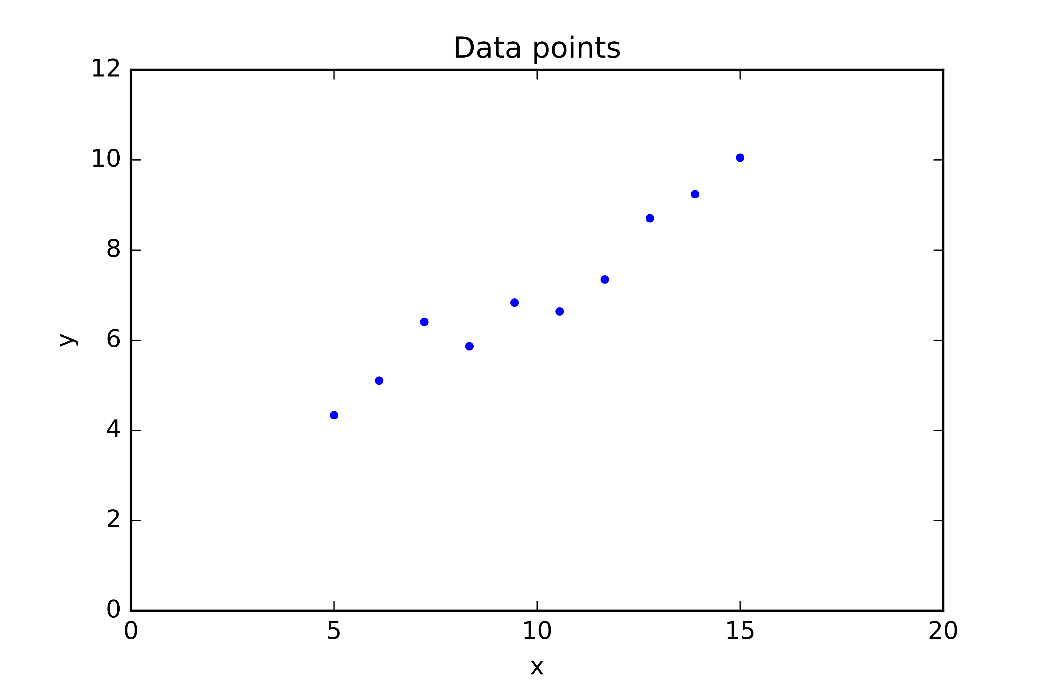
Code
# Generate some data
np.random.seed(0)

m_true = .75
c_true = 1

x = np.hstack([np.linspace(3, 5, 5), np.linspace(7, 8, 5)])
y = m_true * x + c_true + np.random.rand(len(x))

#x = np.linspace(1,9,10)
#y = np.ones(10)+5

#y = np.linspace(1,9,10)
#x = np.ones(10)+5

data = np.vstack([x, y]).T
n = data.shape[0]

plt.figure(figsize=(7,7))
plt.scatter(data[:,0], data[:,1], c='red', alpha=0.9)
plt.xlim([0,10])
plt.ylim([0,10])
plt.title('Generating some points from a line')
Text(0.5, 1.0, 'Generating some points from a line')

print(f'data =\n{data}')
n = data.shape[0]
print(f'Number of data items = {n}')
data =
[[3.         3.7988135 ]
 [3.5        4.34018937]
 [4.         4.60276338]
 [4.5        4.91988318]
 [5.         5.1736548 ]
 [7.         6.89589411]
 [7.25       6.87508721]
 [7.5        7.516773  ]
 [7.75       7.77616276]
 [8.         7.38344152]]
Number of data items = 10
A = np.ones([n, 2])
A[:,0] = data[:,0]
print(f'A =\n{A}')
A =
[[3.   1.  ]
 [3.5  1.  ]
 [4.   1.  ]
 [4.5  1.  ]
 [5.   1.  ]
 [7.   1.  ]
 [7.25 1.  ]
 [7.5  1.  ]
 [7.75 1.  ]
 [8.   1.  ]]
AtA = np.dot(A.T,A)
print(f'AtA =\n {AtA}')
AtA =
 [[364.375  57.5  ]
 [ 57.5    10.   ]]
AtY = np.dot(A.T, data[:,1].reshape(n,1))
print(f'AtY = \n{AtY}')
AtY =
[[366.83013724]
 [ 59.28266283]]
# m = slope
# c = intercept
m_and_c = np.dot(np.linalg.inv(AtA), AtY)

m = m_and_c[0]
c = m_and_c[1]

print(f'm = {m}')
print(f'c = {c}')
m = [0.76903188]
c = [1.50633297]
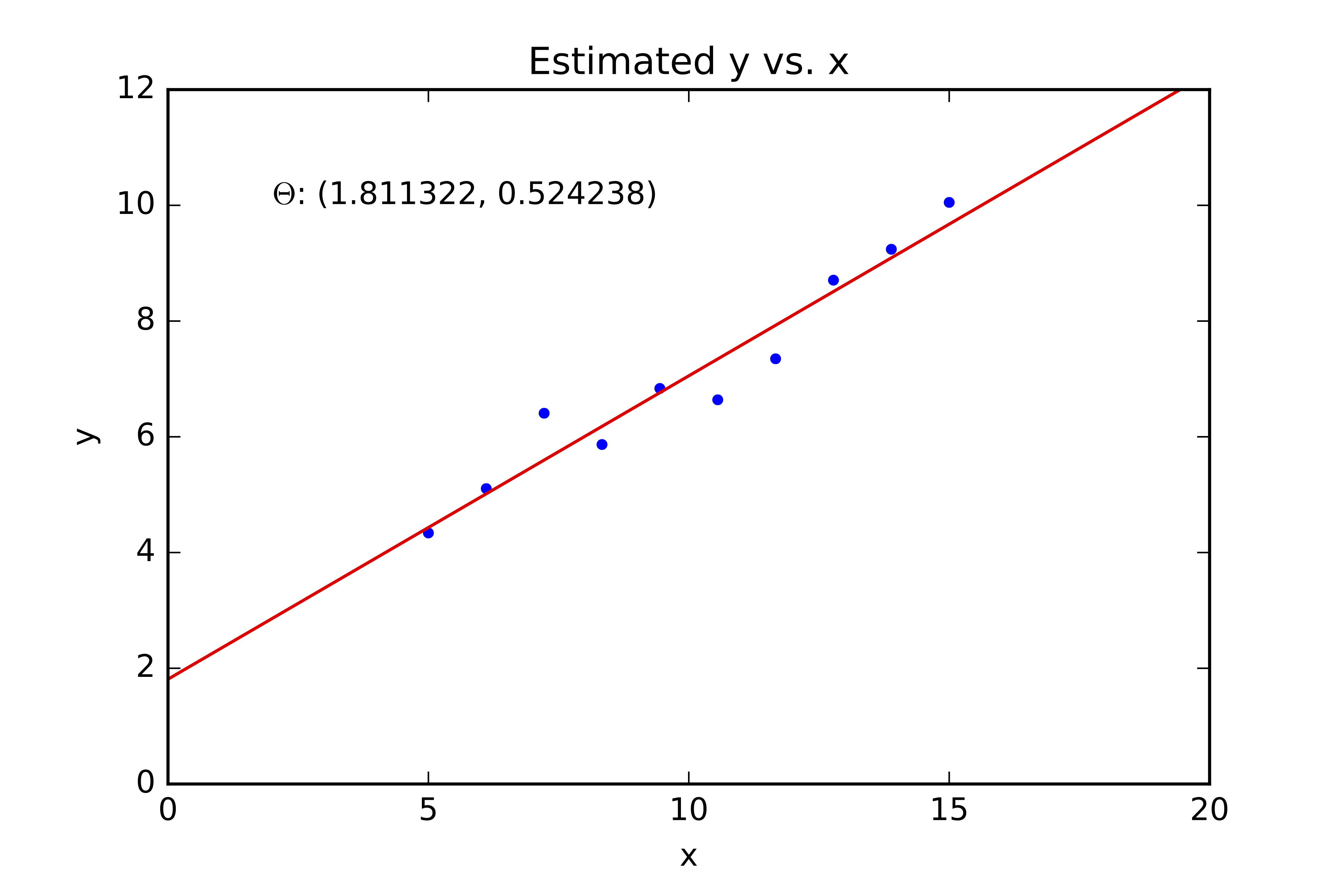
x_plotting = np.linspace(0,10,100)
y_plotting = m * x_plotting + c

plt.figure(figsize=(7,7))
plt.scatter(data[:,0], data[:,1], c='red', alpha=0.9)
plt.plot(x_plotting, y_plotting, 'b-')
plt.xlim([0,10])
plt.ylim([0,10])
plt.title('Line fitted to data using least squares.');

Robust least squares: A detour
# Generate some data
np.random.seed(0)

m_true = .75
c_true = 1

x = np.hstack([np.linspace(3, 5, 5), np.linspace(7, 8, 5)])
y = m_true * x + c_true + np.random.rand(len(x))

# Outliers
y[9] = 1
y[0] = 9

data = np.vstack([x, y]).T
n = data.shape[0]

plt.figure(figsize=(7,7))
plt.scatter(data[:,0], data[:,1], c='red', alpha=0.9)
plt.xlim([0,10])
plt.ylim([0,10])
plt.title('Generating some points from a line');

x, y = data[:,0], data[:,1]

theta = np.polyfit(x, y, 1)
m = theta[0]
c = theta[1]

print(f'c = {c}')
print(f'm = {m}')
c = 6.271945578021885
m = -0.08033126904046155
x_plotting = np.linspace(0,10,100)
y_plotting = m * x_plotting + c

plt.figure(figsize=(7,7))
plt.scatter(data[:,0], data[:,1], c='red', alpha=0.9)
plt.plot(x_plotting, y_plotting, 'b-')
plt.xlim([0,10])
plt.ylim([0,10])
plt.title('The effect of outliers on least squares');

Loss functions
In the discussion below, set $$ e = y_{\mathrm{prediction}} - y_{\mathrm{true}} $$ and $$ z = e^2 $$ In other words, $z$ is error-squared.
The following expressions are pulled out from scipy implementation of least squares. For an in depth discussion, I suggest "Convex Optimization" by Boyd et al, 2004 to the interested reader.
Linear loss
$$ \rho(z) = z $$
Soft L1 loss
$$ \rho(z) = 2 \left(\sqrt{1+z} - 1\right) $$
Huber loss
Generally
$$ \rho(e) = \begin{cases} \frac{1}{2} e^2 & \text{for } |e| \le k \\ k|e| - \frac{1}{2}k^2 & \text{otherwise} \end{cases} $$
Here $k$ is referred to as the tuning constant. Smaller values of $k$ produce more resistance to outliers, but at the expense of lower efficiency when the errors are normally distributed. The tuning constant is generally picked to give reasonably high efficiency in the normal case. Typically, we set $k = 1.345 \sigma$ for the Huber (where $\sigma$ is the standard deviation of the errors) produce 95-percent efficiency when the errors are normal, and still offer protection against outliers.
In scipy.optimize.least_square Huber loss is defined as
$$ \rho(z) = \begin{cases} z & \text{for } z \le 0 \\ 2 \left( \sqrt(1+z) - 1 \right) & \text{otherwise} \end{cases} $$
Cauchy loss
$$ \rho(z) = \ln (1 + z) $$
arctan loss
$$ \rho(z) = \arctan(z) $$
Bisquare
Generally
$$ \rho(e) = \begin{cases} \frac{k^2}{6} \{ 1 - \left[ 1 - \left( \frac{e}{k} \right)^2 \right]^3 \} & \text{for } |e| \le k \\ \frac{k^2}{6} & \text{otherwise} \end{cases} $$
$$ \rho(z) = \frac{z}{z + \sigma^2} $$
Here $\sigma$ is often referred to a scale parameter.
e = np.linspace(-3,3,100)
z = np.square(e)

linear_loss = z
l1_loss = np.abs(e)
soft_l1_loss = 2*(np.power(1+z, 0.5) - 1) # Smooth approx. of l1 loss.
huber_loss = 2*np.power(z, 0.5) - 1
huber_loss[z <= 1] = z[z <= 1]
cauchy_loss = np.log(1 + z)
arctan_loss = np.arctan(z)

scale = 0.1
robust_loss = z / (z + scale**2)

plt.figure(figsize=(15,15))
plt.subplot(331)
plt.title('Linear loss')
plt.ylim(0,10)
plt.grid()
plt.plot(e, linear_loss, label='Linear loss')
plt.subplot(332)
plt.grid()
plt.ylim(0,10)
plt.title('L1 loss')
plt.plot(e, l1_loss, label='L1 loss')
plt.subplot(333)
plt.grid()
plt.ylim(0,10)
plt.title('Soft L1 loss')
plt.plot(e, soft_l1_loss, label='Soft L1 loss')
plt.subplot(334)
plt.grid()
plt.ylim(0,10)
plt.title('Huber loss')
plt.plot(e, huber_loss, label='Huber loss')
plt.subplot(335)
plt.grid()
plt.ylim(0,10)
plt.title('Cauchy loss')
plt.plot(e, cauchy_loss, label='Cauchy loss')
plt.subplot(336)
plt.grid()
plt.ylim(0,10)
plt.title('Arctan loss')
plt.plot(e, arctan_loss, label='Arctan loss')
plt.subplot(337)
plt.grid()
plt.ylim(0,10)
plt.title('?Loss')
plt.plot(e, robust_loss, label='Robust loss')
plt.subplot(338)
plt.grid()
plt.title('?Loss (Rescaled y-axis)')
plt.plot(e, z / (z + 2**2), label=r'$\sigma=2$')
plt.plot(e, z / (z + 1**2), label=r'$\sigma=1$')
plt.plot(e, z / (z + .5**2), label=r'$\sigma=.5$')
plt.plot(e, z / (z + .25**2), label=r'$\sigma=.25$')
plt.plot(e, z / (z + .1**2), label=r'$\sigma=.1$')
plt.legend();

# Generate some data
np.random.seed(0)

m_true = .75
c_true = 1

x = np.hstack([np.linspace(1, 5, 50), np.linspace(7, 10, 50)])
y = m_true * x + c_true + np.random.rand(len(x))*.2

data = np.vstack([x, y]).T
n = data.shape[0]

outlier_percentage = 50
ind = (np.random.rand(int(n*outlier_percentage/100))*n).astype('int')
data[ind, 1] = np.random.rand(len(ind))*9

plt.figure(figsize=(7,7))
plt.scatter(data[:,0], data[:,1], c='red', alpha=0.9)
plt.xlim([0,10])
plt.ylim([0,10])
plt.title('Noisy data');

theta_guess = [1, 1] # Need an intial guess

# Available losses
losses = [
    'linear',
    'soft_l1',
    'huber',
    'cauchy',
    'arctan'
]
loss_id = 4  # Pick a loss
def line_fitting_errors(x, data):
    m = x[0]
    c = x[1]
    y_predicted = m * data[:,0] + c
    e = y_predicted - data[:,1]
    return e
# Non-linear least square fitting
from scipy.optimize import least_squares
retval = least_squares(line_fitting_errors, theta_guess, loss=losses[loss_id], args=[data])
print(f'Reasons for stopping: {retval["message"]}')
print(f'Success: {retval["success"]}')
theta = retval['x']
print(f'#data = {n}')
print(f'theta = {theta}')
Reasons for stopping: `ftol` termination condition is satisfied.
Success: True
#data = 100
theta = [0.73475407 1.15731305]
def draw_line(theta, ax, **kwargs):
    m = theta[0]
    c = theta[1]

    xmin, xmax = ax.get_xbound()

    ymin = m * xmin + c
    ymax = m * xmax + c

    l = mlines.Line2D([xmin, xmax], [ymin,ymax], **kwargs)
    ax.add_line(l)
plt.figure(figsize=(7,7))
ax = plt.gca()
plt.scatter(data[:,0], data[:,1], c='red', alpha=0.9)
plt.xlim([0,10])
plt.ylim([0,10])
plt.title(f'Non linear least squares.  Loss = {losses[loss_id]}')
draw_line(theta, ax, c='black', linewidth='3');

Model fitting
- Robust least square fitting is a non-linear optimization problem, which must be solved iteratively
Key Takeaway 1
- Model
- Parameters, and optionally hyper-parameters
- Mechanism to determine model fitness
- Loss
- Model fitting
- Searching model parameters that results in the "best" model fitness or the "lowest" loss
- Even for simple problems, it is not always possible to fit the model using an analytical solution
- For neural networks, we often use some variant of gradient descent
- The ability to compute gradient of loss w.r.t. model paramters (and inputs)
Linear least squares in higher dimensions
$ \newcommand{\bx}{\mathbf{x}} \newcommand{\bX}{\mathbf{X}} \newcommand{\by}{\mathbf{y}} \newcommand{\bY}{\mathbf{Y}} $
Input feature: $\mathbf{x}^{(i)} = \left(1, x_{1}^{(i)}, x_{2}^{(i)}, \cdots, x_{M}^{(i)} \right)^T$.
For this discussion, we assume $x_{0}^{(i)}=1$ (just to simplify mathematical notation).
Target feature: $y^{(i)}$
Parameters: $\theta = \left( \theta_0, \theta_1, \cdots, \theta_M \right)^T \in \mathbb{R}^{(M+1)}$
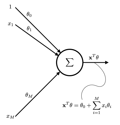
Model: $f(\bx) = \bx^T \theta$
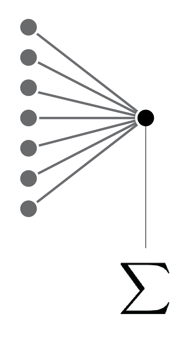
Linear regression and perceptron ... each connection represents a model parameter.
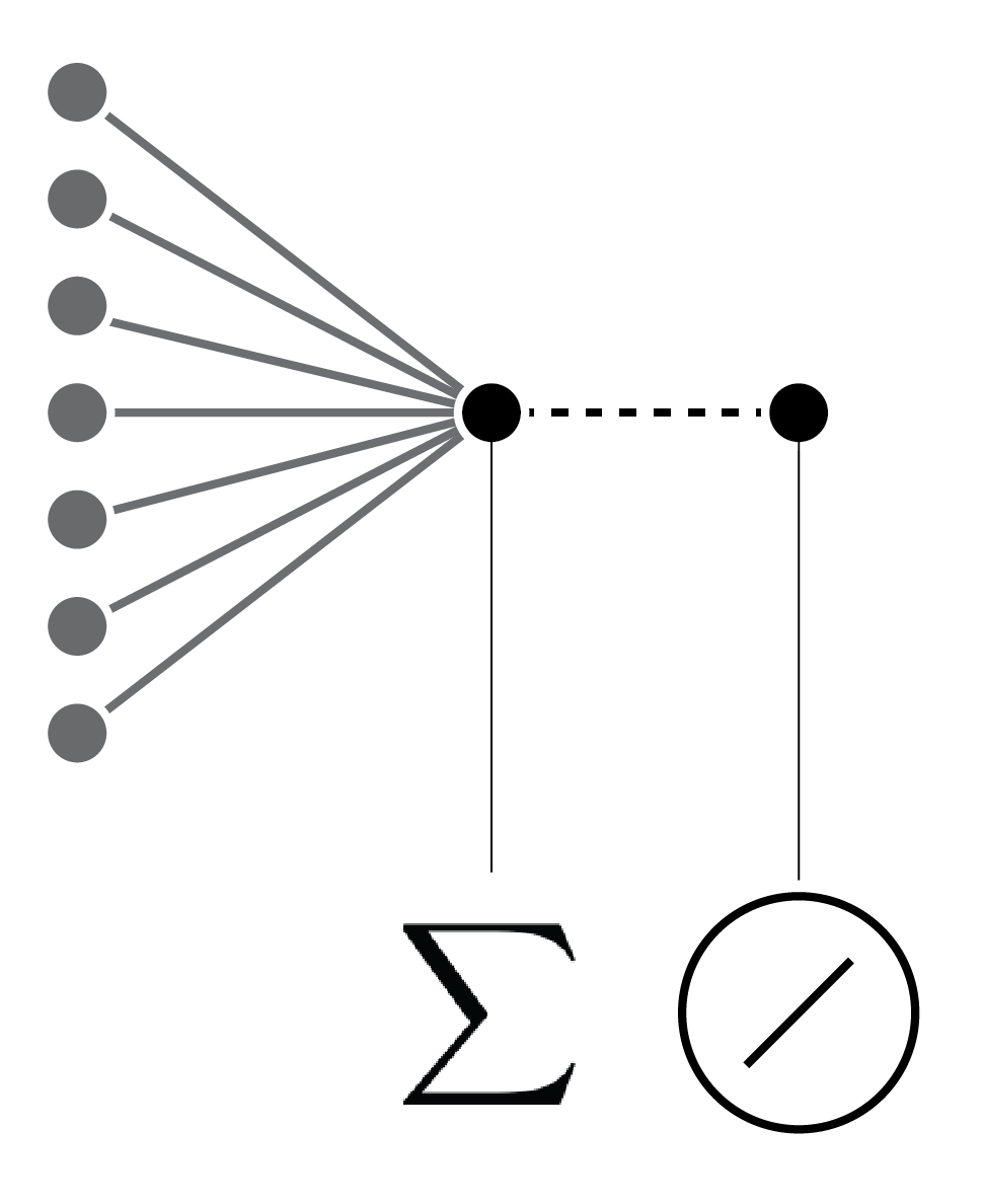
Linear regression and perceptron ... each connection represents a model parameter. With a linear activation function.
Loss: $C(\theta) = (\bY - \bX \theta)^T (\bY - \bX \theta)$
Design matrix:
$$ \bX = \left[ \begin{array}{ccc} - & \bx_1^T & -\\ - & \bx_2^T & -\\ & \vdots & \\ - & \bx_N^T & - \end{array} \right] \in \mathbb{R}^{N \times (M+1)} $$
Output:
$$ \bY = \left[ \begin{array}{c} y_1 \\ y_2 \\ \vdots \\ y_N \end{array} \right] \in \mathbb{R}^{N \times 1} $$
Solution:
Solve $\theta$ by setting $\frac{\partial C}{\partial \theta} = 0$
Solution is $$\hat \theta = (\bX^T \bX)^{-1} \bX^T \bY$$Derivation: you can find the derivation here.
Beyond lines and planes
How can we construct more complex models?
There are many ways to make linear models more powerful while retaining their nice mathematical properties:
- By using non-linear, non-adaptive basis functions, we can get generalized linear models that learn non-linear mappings from input to output but are linear in their parameters (only the linear part of the model learns).
- By using kernel methods we can handle expansions of the raw data that use a huge number of non-linear, non-adaptive basis functions. simple case.
- Linear models do have fundamental limitations, and these can't be used to solve all our AI problems. (from R. Urtasun)
Basis functions
- It is possible to introduce non-linearity in the system by using basis functions $\phi(.)$ as follows:
$$ f(\bx) = \mathbf{\phi}(\bx)^T \theta $$
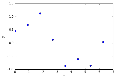
Example - Using a cubic polynomial
For a cubic polynomial (in 1D)
$\phi_0(x) = 1$
$\phi_1(x) = x$
$\phi_2(x) = x^2$
$\phi_3(x) = x^3$
Then
$$ f(x) = \left[ \begin{array}{cccc} \phi_0(x) & \phi_1(x) & \phi_2(x) & \phi_3(x) \end{array} \right] \left[ \begin{array}{c} \theta_0 \\ \theta_1 \\ \theta_2 \\ \theta_3 \end{array} \right] $$
- Using the basis functions, the loss can be written as
$$ C(\theta) = \left(\bY - \Phi^T \theta \right)^T \left(\bY - \Phi^T \theta \right) $$
- And the solution is
$$ \hat \theta = (\Phi^T \Phi)^{-1} \Phi^T \bY $$
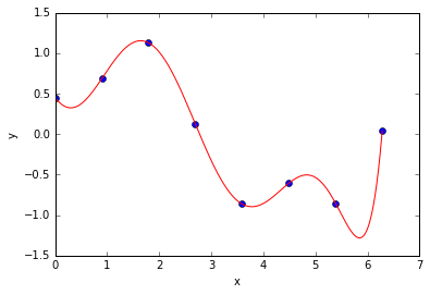
- Note that the model is still linear in $\theta$. We can still use the same least squares loss and use the same technique that we used for fitting a line in 1D to fit the polynomial.
Example basis functions
Polynomials (as seen before)
Sigmoid
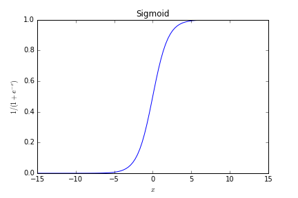
Sigmoid function
Gaussian
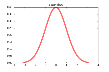
Gaussian function
Key Takeaway 2
- It is possible to use basis functions to develop models capable of dealing with non-linearities present in the data
- Neural networks can be seen as using basis functions as well; however, there is a key difference, neural networks can also learn the "parameters" of the basis functions themselves.
- Linear regression models discussed above only learns the parameters $\theta$, i.e., the basis functions themselves are fixed.
Regularization
- Increasing input features or model parameters can increase model complexity
- We need an automatic way to select appropriate model complexity
- Regularization is the standard technique that is used to achieve this goal
- Eg., use the following loss function that penalize squared parameters: $$ C(\theta) = \left( \by - \bX \theta \right)^T \left( \by - \bX \theta \right) + \delta^2 \theta^T \theta $$
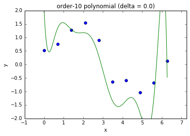
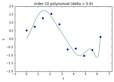
Model complexity and fit
- This is referred to as ridge regression in statistics.
Key Takeaway 3
- Regularization is necessary to reduce generalization error without effecting training error.
- Without regularization a complex model will most likely overfit training data, leading to poor performance on test data.
- Extra constraints and penalties
- Prior knowledge
Q. What about neural networks? How do we deal with model complexity in neural networks?
A network view of regression and logistic regression
- Linear regression and logistic regression topics provide an excellent opportunity to study and understand the concepts underpinning neural networks
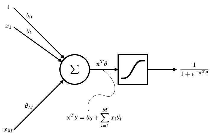
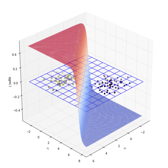
Logisitc regression
- Network view of logistic regression
- By changing the activation function to sigmoid and using the cross-entropy loss instead the least-squares loss that we use for linear regression, we are able to perform binary classification.
Binary classification
Given a point $\mathbf{x}^{(*)}$, classify using the following rule:
$$ \begin{equation} y^{(*)} = \begin{cases} 1 & \mathrm{ if\ } \mathrm{Pr}(y|\bx^{(*)},\theta) \ge 0.5 \\ 0 & \mathrm{ otherwise} \end{cases} \end{equation} $$
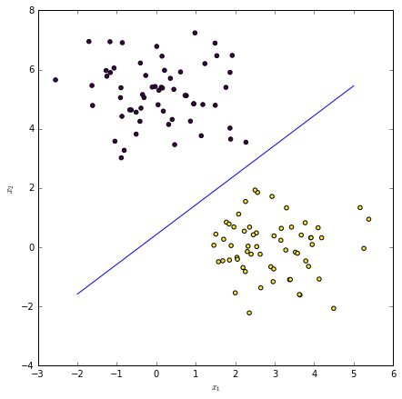
The decision boundary is $\mathbf{x}^T \theta = 0$. Recall that this is where sigmoid function is $0.5$.
Summary
- Linear regression
- Model fitting by optimizing some objective function
- The need for gradient-based iterative methods for model fitting when analytical solution is not readily available
- Model complexity
- The need for regularization
- A network view of linear regression (for regression) and logistic regression (for classification)
- Connections to both perceptron and neural networks