Convolutional Networks
Faisal Qureshi
http://www.vclab.ca
Lesson Plan
- Convolutional Networks
- Convolution
- Pooling layers
- Dilated convolutions
- Common architecture
- GoogLeNet
- ResNet
- Densenet
- Squeeze-and-Excitation network
- ConvNext
Convolutional networks for computer vision tasks
Task: We want to classify the following image
import cv2
import matplotlib.pyplot as plt

img = cv2.imread('./convnet/1.jpeg', 0)
plt.figure(figsize=(10,8))
plt.imshow(img, cmap='gray')
plt.xlabel('width')
plt.xticks([])
plt.ylabel('height')
plt.yticks([])
plt.title(f'Image dimensions: {img.shape[0]} x {img.shape[1]}.  #pixels: {img.shape[0] * img.shape[1]}');

Classical neural networks for computer vision tasks
- Q. How many paramters per hidden layer unit?
- Computational issues
- Poor performance
- The model is prone to overfitting
- Model capacity issues
Convolutional neural network
- David Hubel and Torsten Wiesel studied cat visual cortex and showed that visual information goes through a series of processing steps: 1) edge detection; 2) edge combination; 3) motion perception; etc. (Hubeland Wiesel, 1959)
- Neurons are spatially localized
- Topographic feature maps
- Hierarchical feature processing
- Convolutional layers achieve these properties
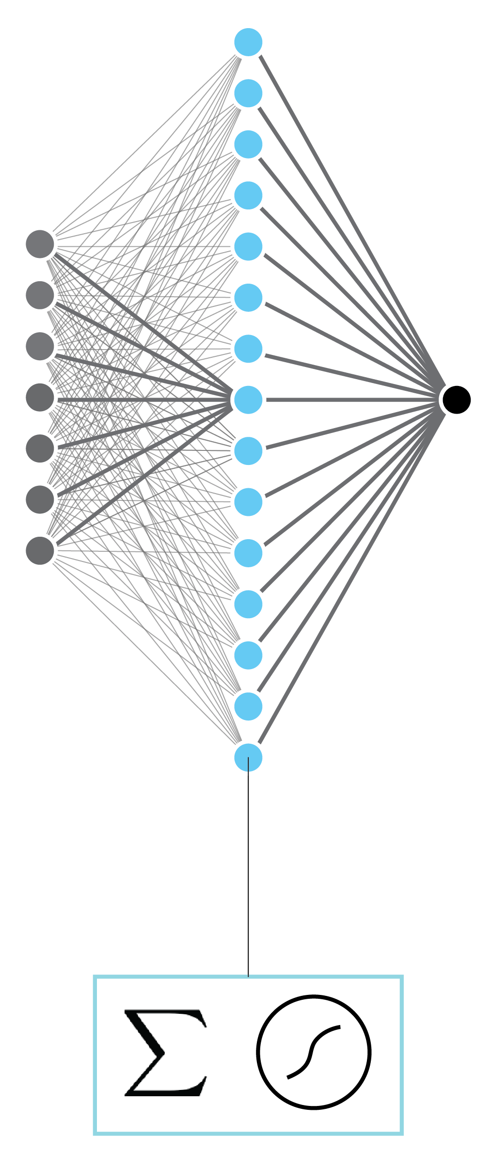
- Each output unit is a linear function of a localized subset of input units
- Same linear transformation is applied at each location
- Local features detection is translation invariant
- Convolutional layers provide architectural constraints
- Number of parameters depend upon kernel sizes and not the size of the input
- Inductive bias
- Examples:
- Architectural constraints
- Image augmentation
- Regularization
- Examples:
- The first few layers are convolution layers, and the last few layers are fully connected layers
- Q. Why?
- The convolutional layers are compute heavy, but have fewer parameters
- The fully connected layer have far more parameters, but these are easy to compute
- Q. Why?
General idea
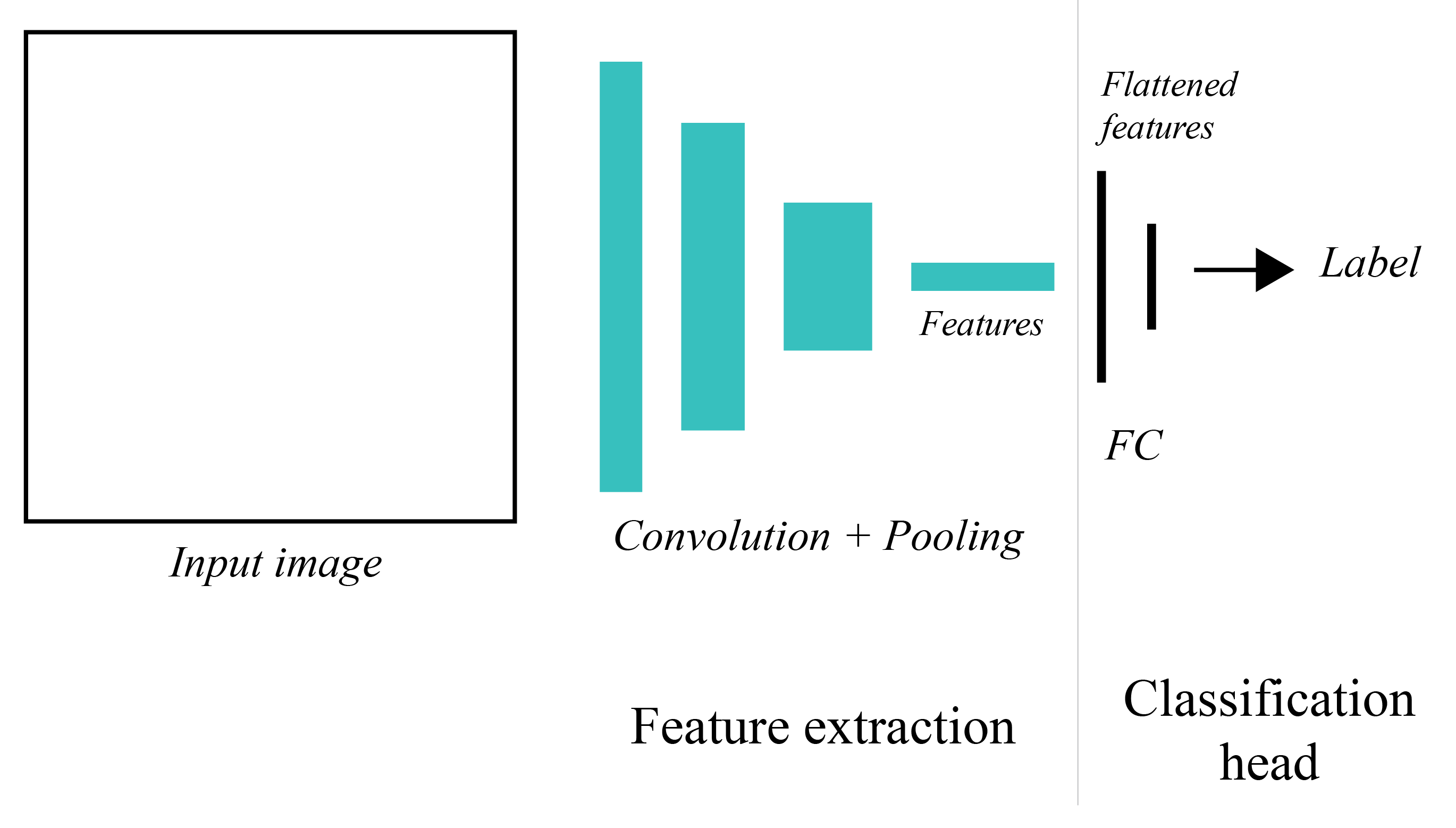
- Generally speaking we can interpret convolutional deep networks as composed of two parts: 1) a (latent) feature extractor and 2) task head.
- Feature extractor learns to construct powerful representations given an input. These representations are well-suited to the task at hand.
Convolution
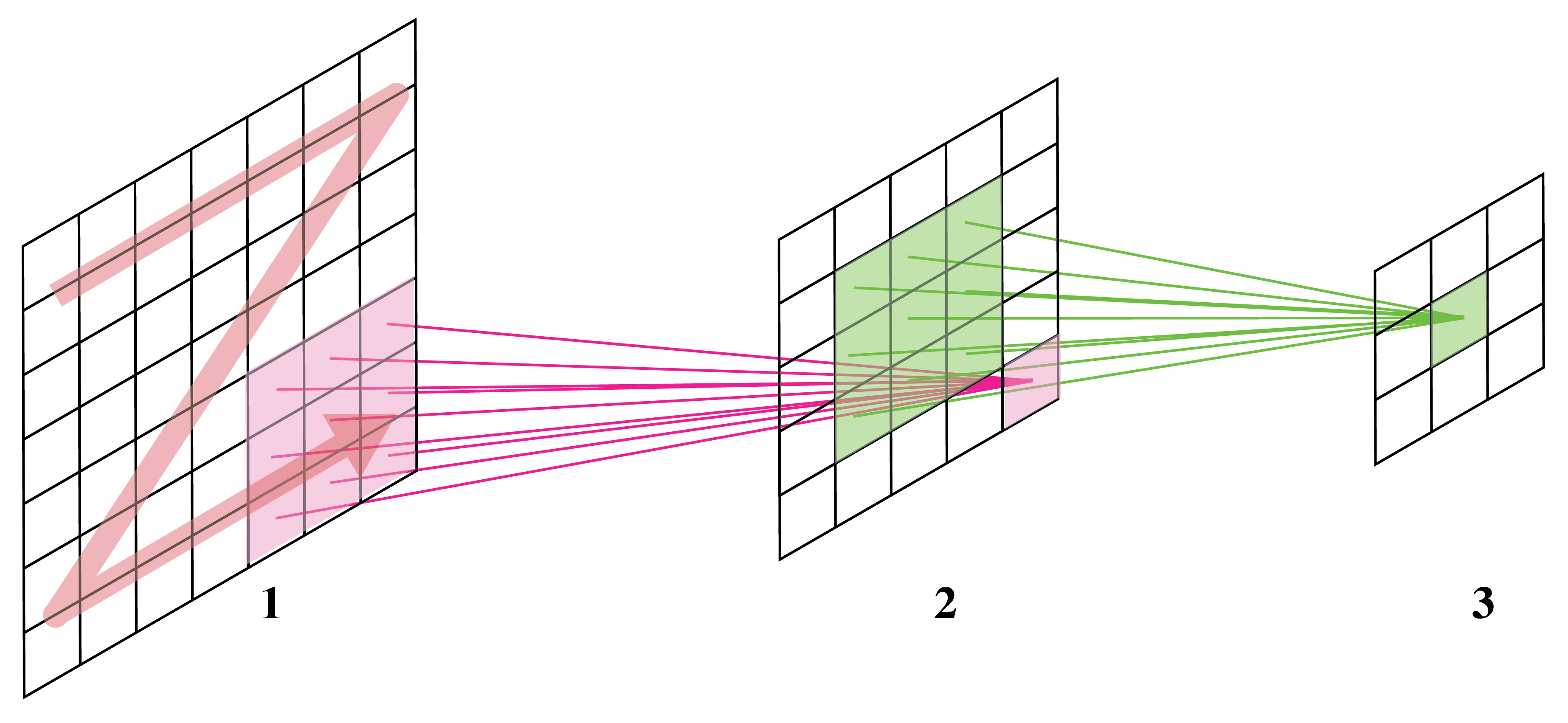
- In a nutshell: point-wise multiplication and sum
$$ (\mathbf{f} \ast \mathbf{k} )_i = \sum_{k \in [-w,w]} \mathbf{f}(i - k) \mathbf{h}(k) $$
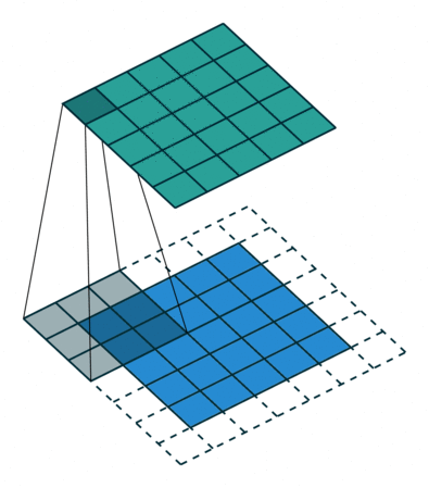
2D convolution using kernel size 3, stride 1, and padding 1. Figure from towardsdatascience.com
Exercise: computing a 1D convolution (from scratch)
Compute $\mathbf{f} \ast \mathbf{h}$ given
$$ \mathbf{f} = \left[ \begin{array}{cccccccc} 1 & 3 & 4 & 1 & 10 & 3 & 0 & 1 \end{array} \right] $$
and
$$ \mathbf{h} = \left[ \begin{array}{ccc} 1 & 0 & -1 \end{array}\right] $$
import numpy as np

f = np.array([1,3,4,1,10,3,0,1])
h = np.array([1,0,-1])
width = 1
result = np.ones(len(f)-2*width)   # Array to store computed moving averages
for i in range(len(result)):
    centre = i + width
    result[i] = np.dot(h[::-1], f[centre-width:centre+width+1]) # Note the flip
print(f'signal f:\t\t{f}')
print(f'kernel h:\t\t{h}')
print(f'convolution (f*h):\t{result}')
signal f:		[ 1  3  4  1 10  3  0  1]
kernel h:		[ 1  0 -1]
convolution (f*h):	[  3.  -2.   6.   2. -10.  -2.]
Dealing with edges
- Clipping
- Replication
- Symmetric padding
- Circular padding
Convolutions as matrix-vector multiplication
- Exercise: Describe 1D convolution as a matrix-vector multiplication.
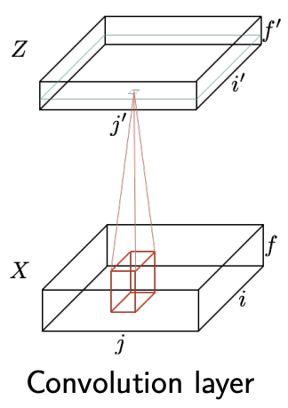
Convolution layer
We can define the convolution layer used in deep networks as follows
$$ \mathbf{z}_{i',j',f'} = b_{f'} + \sum_{i=1}^{H_f} \sum_{j=1}^{W_f} \sum_{f=1}^{F} \mathbf{x}_{i'+i-1,j'+j-1,f} \theta_{ijff'}. $$
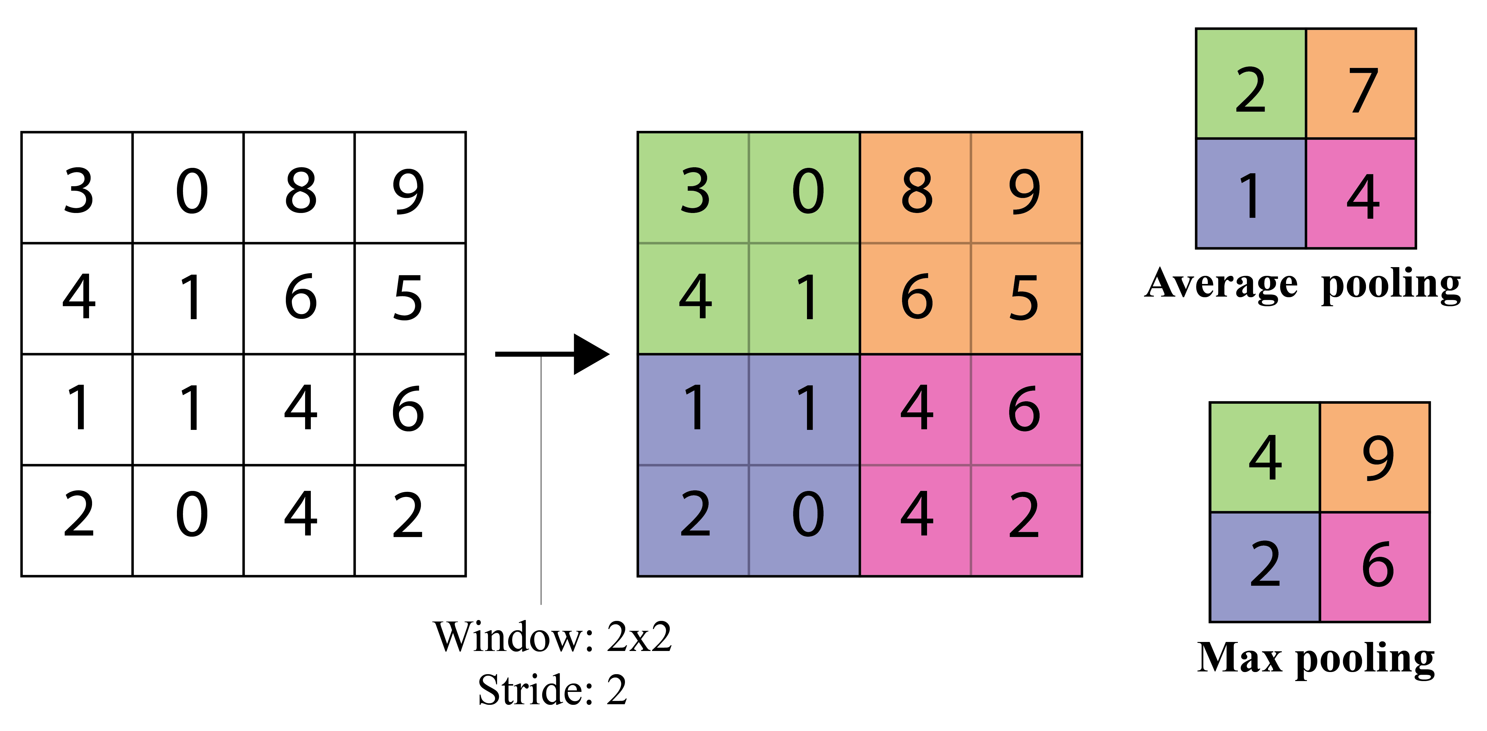
Pooling layers
- Pooling layers are commonly used after convoluational layers
- Decrease feature dimensions
- Create some invariance to shifts
- Average pooling $$ h_k(x,y,c) = \frac{1}{\mathcal{N}(x,y)} \sum_{(i,j) \in \mathcal{N}_(x,y)} h_{k-1}(i,j,c) $$
- Maxpooling $$ \DeclareMathOperator*{\max}{max} h_k(x,y,c) = \max_{(i,j) \in \mathcal{N}(x,y)} h_{k-1}(i,j,c) $$
- Springenberg et al. 2015 (ICLR workshops)
maxpooling can simply be replaced by a convolutional layer with increased stride without loss in accuracy on several image recognition benchmarks
Other types of convolutions
Dilated convolution
- Atrous convolutions
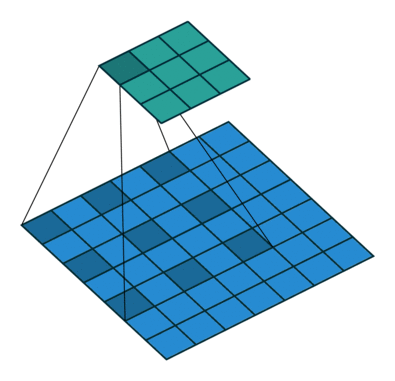
Dilated convolution. 2D convolution using a 3 kernel with a dilation rate of 2 and no padding. Figure from towardsdatascience.com
import torchvision
import torchvision.models as m
import pprint as pp
print(f'torchvision\nVERSION: {torchvision.__version__}')
print('MODELS:')
pp.pprint([x for x in dir(m) if x[0] != '_'])
torchvision
VERSION: 0.23.0
MODELS:
['AlexNet',
 'AlexNet_Weights',
 'ConvNeXt',
 'ConvNeXt_Base_Weights',
 'ConvNeXt_Large_Weights',
 'ConvNeXt_Small_Weights',
 'ConvNeXt_Tiny_Weights',
 'DenseNet',
 'DenseNet121_Weights',
 'DenseNet161_Weights',
 'DenseNet169_Weights',
 'DenseNet201_Weights',
 'EfficientNet',
 'EfficientNet_B0_Weights',
 'EfficientNet_B1_Weights',
 'EfficientNet_B2_Weights',
 'EfficientNet_B3_Weights',
 'EfficientNet_B4_Weights',
 'EfficientNet_B5_Weights',
 'EfficientNet_B6_Weights',
 'EfficientNet_B7_Weights',
 'EfficientNet_V2_L_Weights',
 'EfficientNet_V2_M_Weights',
 'EfficientNet_V2_S_Weights',
 'GoogLeNet',
 'GoogLeNetOutputs',
 'GoogLeNet_Weights',
 'Inception3',
 'InceptionOutputs',
 'Inception_V3_Weights',
 'MNASNet',
 'MNASNet0_5_Weights',
 'MNASNet0_75_Weights',
 'MNASNet1_0_Weights',
 'MNASNet1_3_Weights',
 'MaxVit',
 'MaxVit_T_Weights',
 'MobileNetV2',
 'MobileNetV3',
 'MobileNet_V2_Weights',
 'MobileNet_V3_Large_Weights',
 'MobileNet_V3_Small_Weights',
 'RegNet',
 'RegNet_X_16GF_Weights',
 'RegNet_X_1_6GF_Weights',
 'RegNet_X_32GF_Weights',
 'RegNet_X_3_2GF_Weights',
 'RegNet_X_400MF_Weights',
 'RegNet_X_800MF_Weights',
 'RegNet_X_8GF_Weights',
 'RegNet_Y_128GF_Weights',
 'RegNet_Y_16GF_Weights',
 'RegNet_Y_1_6GF_Weights',
 'RegNet_Y_32GF_Weights',
 'RegNet_Y_3_2GF_Weights',
 'RegNet_Y_400MF_Weights',
 'RegNet_Y_800MF_Weights',
 'RegNet_Y_8GF_Weights',
 'ResNeXt101_32X8D_Weights',
 'ResNeXt101_64X4D_Weights',
 'ResNeXt50_32X4D_Weights',
 'ResNet',
 'ResNet101_Weights',
 'ResNet152_Weights',
 'ResNet18_Weights',
 'ResNet34_Weights',
 'ResNet50_Weights',
 'ShuffleNetV2',
 'ShuffleNet_V2_X0_5_Weights',
 'ShuffleNet_V2_X1_0_Weights',
 'ShuffleNet_V2_X1_5_Weights',
 'ShuffleNet_V2_X2_0_Weights',
 'SqueezeNet',
 'SqueezeNet1_0_Weights',
 'SqueezeNet1_1_Weights',
 'SwinTransformer',
 'Swin_B_Weights',
 'Swin_S_Weights',
 'Swin_T_Weights',
 'Swin_V2_B_Weights',
 'Swin_V2_S_Weights',
 'Swin_V2_T_Weights',
 'VGG',
 'VGG11_BN_Weights',
 'VGG11_Weights',
 'VGG13_BN_Weights',
 'VGG13_Weights',
 'VGG16_BN_Weights',
 'VGG16_Weights',
 'VGG19_BN_Weights',
 'VGG19_Weights',
 'ViT_B_16_Weights',
 'ViT_B_32_Weights',
 'ViT_H_14_Weights',
 'ViT_L_16_Weights',
 'ViT_L_32_Weights',
 'VisionTransformer',
 'Weights',
 'WeightsEnum',
 'Wide_ResNet101_2_Weights',
 'Wide_ResNet50_2_Weights',
 'alexnet',
 'convnext',
 'convnext_base',
 'convnext_large',
 'convnext_small',
 'convnext_tiny',
 'densenet',
 'densenet121',
 'densenet161',
 'densenet169',
 'densenet201',
 'detection',
 'efficientnet',
 'efficientnet_b0',
 'efficientnet_b1',
 'efficientnet_b2',
 'efficientnet_b3',
 'efficientnet_b4',
 'efficientnet_b5',
 'efficientnet_b6',
 'efficientnet_b7',
 'efficientnet_v2_l',
 'efficientnet_v2_m',
 'efficientnet_v2_s',
 'get_model',
 'get_model_builder',
 'get_model_weights',
 'get_weight',
 'googlenet',
 'inception',
 'inception_v3',
 'list_models',
 'maxvit',
 'maxvit_t',
 'mnasnet',
 'mnasnet0_5',
 'mnasnet0_75',
 'mnasnet1_0',
 'mnasnet1_3',
 'mobilenet',
 'mobilenet_v2',
 'mobilenet_v3_large',
 'mobilenet_v3_small',
 'mobilenetv2',
 'mobilenetv3',
 'optical_flow',
 'quantization',
 'regnet',
 'regnet_x_16gf',
 'regnet_x_1_6gf',
 'regnet_x_32gf',
 'regnet_x_3_2gf',
 'regnet_x_400mf',
 'regnet_x_800mf',
 'regnet_x_8gf',
 'regnet_y_128gf',
 'regnet_y_16gf',
 'regnet_y_1_6gf',
 'regnet_y_32gf',
 'regnet_y_3_2gf',
 'regnet_y_400mf',
 'regnet_y_800mf',
 'regnet_y_8gf',
 'resnet',
 'resnet101',
 'resnet152',
 'resnet18',
 'resnet34',
 'resnet50',
 'resnext101_32x8d',
 'resnext101_64x4d',
 'resnext50_32x4d',
 'segmentation',
 'shufflenet_v2_x0_5',
 'shufflenet_v2_x1_0',
 'shufflenet_v2_x1_5',
 'shufflenet_v2_x2_0',
 'shufflenetv2',
 'squeezenet',
 'squeezenet1_0',
 'squeezenet1_1',
 'swin_b',
 'swin_s',
 'swin_t',
 'swin_transformer',
 'swin_v2_b',
 'swin_v2_s',
 'swin_v2_t',
 'vgg',
 'vgg11',
 'vgg11_bn',
 'vgg13',
 'vgg13_bn',
 'vgg16',
 'vgg16_bn',
 'vgg19',
 'vgg19_bn',
 'video',
 'vision_transformer',
 'vit_b_16',
 'vit_b_32',
 'vit_h_14',
 'vit_l_16',
 'vit_l_32',
 'wide_resnet101_2',
 'wide_resnet50_2']
vgg16 = m.vgg16()
print(vgg16)
VGG(
  (features): Sequential(
    (0): Conv2d(3, 64, kernel_size=(3, 3), stride=(1, 1), padding=(1, 1))
    (1): ReLU(inplace=True)
    (2): Conv2d(64, 64, kernel_size=(3, 3), stride=(1, 1), padding=(1, 1))
    (3): ReLU(inplace=True)
    (4): MaxPool2d(kernel_size=2, stride=2, padding=0, dilation=1, ceil_mode=False)
    (5): Conv2d(64, 128, kernel_size=(3, 3), stride=(1, 1), padding=(1, 1))
    (6): ReLU(inplace=True)
    (7): Conv2d(128, 128, kernel_size=(3, 3), stride=(1, 1), padding=(1, 1))
    (8): ReLU(inplace=True)
    (9): MaxPool2d(kernel_size=2, stride=2, padding=0, dilation=1, ceil_mode=False)
    (10): Conv2d(128, 256, kernel_size=(3, 3), stride=(1, 1), padding=(1, 1))
    (11): ReLU(inplace=True)
    (12): Conv2d(256, 256, kernel_size=(3, 3), stride=(1, 1), padding=(1, 1))
    (13): ReLU(inplace=True)
    (14): Conv2d(256, 256, kernel_size=(3, 3), stride=(1, 1), padding=(1, 1))
    (15): ReLU(inplace=True)
    (16): MaxPool2d(kernel_size=2, stride=2, padding=0, dilation=1, ceil_mode=False)
    (17): Conv2d(256, 512, kernel_size=(3, 3), stride=(1, 1), padding=(1, 1))
    (18): ReLU(inplace=True)
    (19): Conv2d(512, 512, kernel_size=(3, 3), stride=(1, 1), padding=(1, 1))
    (20): ReLU(inplace=True)
    (21): Conv2d(512, 512, kernel_size=(3, 3), stride=(1, 1), padding=(1, 1))
    (22): ReLU(inplace=True)
    (23): MaxPool2d(kernel_size=2, stride=2, padding=0, dilation=1, ceil_mode=False)
    (24): Conv2d(512, 512, kernel_size=(3, 3), stride=(1, 1), padding=(1, 1))
    (25): ReLU(inplace=True)
    (26): Conv2d(512, 512, kernel_size=(3, 3), stride=(1, 1), padding=(1, 1))
    (27): ReLU(inplace=True)
    (28): Conv2d(512, 512, kernel_size=(3, 3), stride=(1, 1), padding=(1, 1))
    (29): ReLU(inplace=True)
    (30): MaxPool2d(kernel_size=2, stride=2, padding=0, dilation=1, ceil_mode=False)
  )
  (avgpool): AdaptiveAvgPool2d(output_size=(7, 7))
  (classifier): Sequential(
    (0): Linear(in_features=25088, out_features=4096, bias=True)
    (1): ReLU(inplace=True)
    (2): Dropout(p=0.5, inplace=False)
    (3): Linear(in_features=4096, out_features=4096, bias=True)
    (4): ReLU(inplace=True)
    (5): Dropout(p=0.5, inplace=False)
    (6): Linear(in_features=4096, out_features=1000, bias=True)
  )
)
Common architectures
- Multiple feed-forward passes
- Inception module
- An inception module aims to approximate local sparse structure in a CNN by using filters of different sizes (within the same block) whose output is concatenated and passed on to the next stage
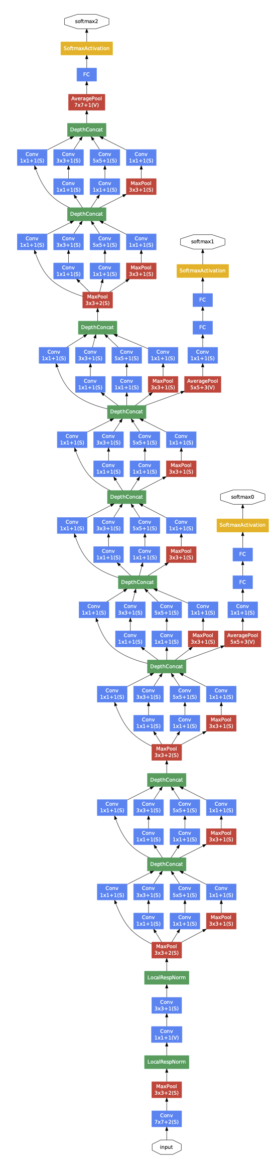
Inception layer
- Acts as a bottleneck layer
- 1-by-1 convolutional layers are used to reduce feature channels
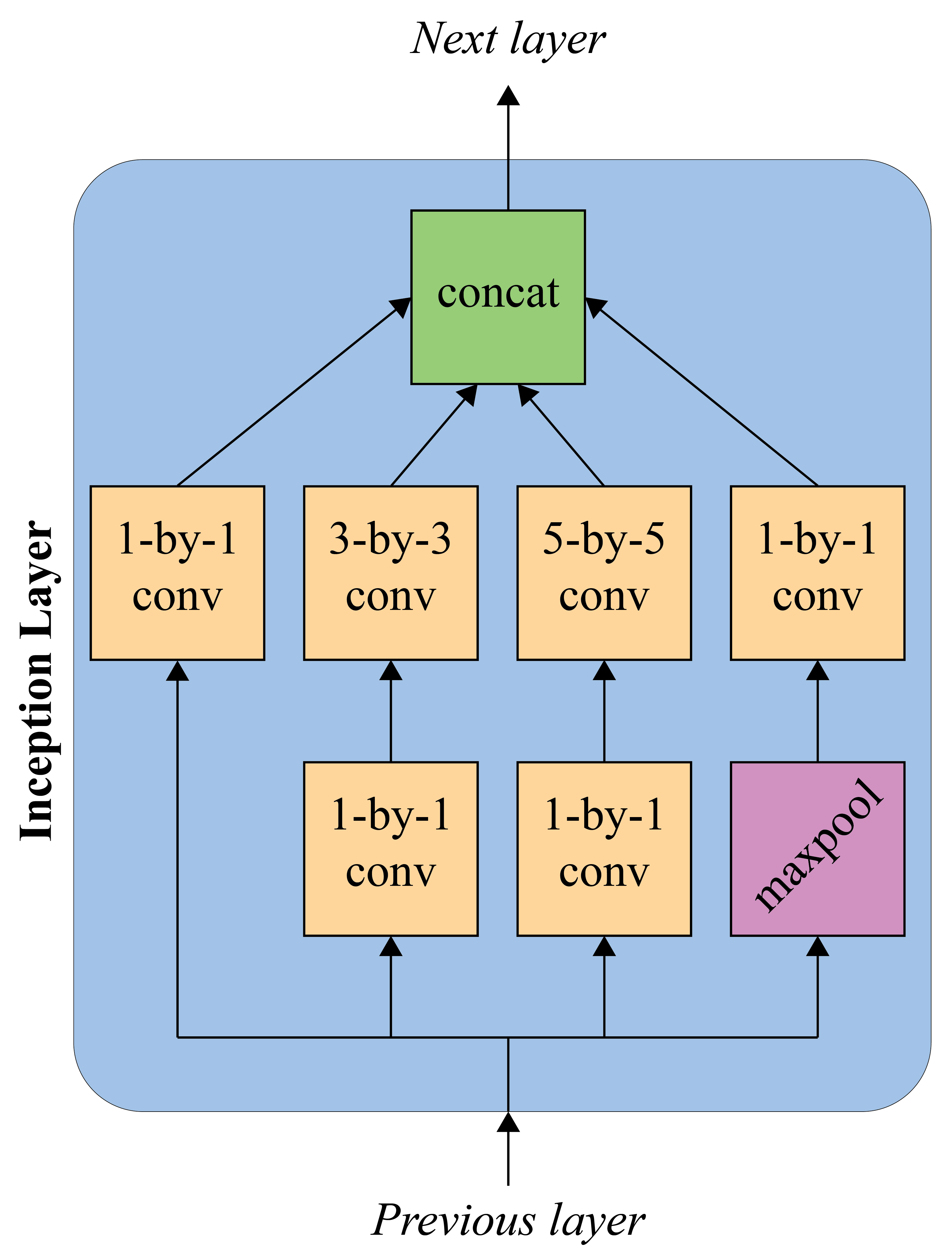
Inception layer (simplified). Each conv is followed by a non-linear activation.
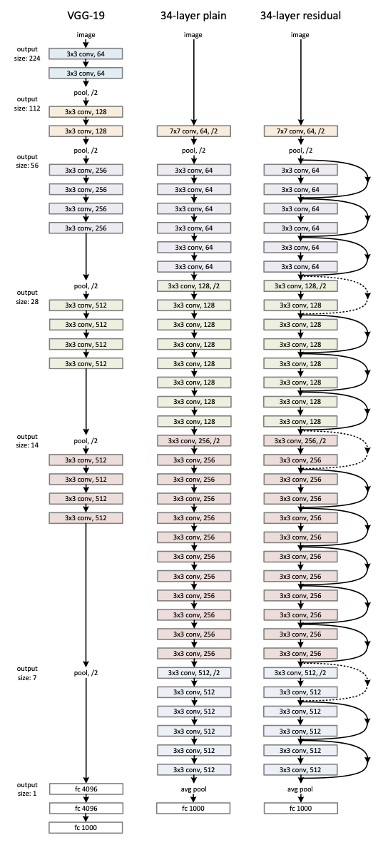
Left: the VGG-19 model (19.6 billion FLOPs) as a reference. Middle: a plain network with 34 parameter layers (3.6 billion FLOPs). Right: a residual network with 34 parameter layers (3.6 billion FLOPs). The dotted shortcuts increase dimensions. Figure from He et al. 2016.
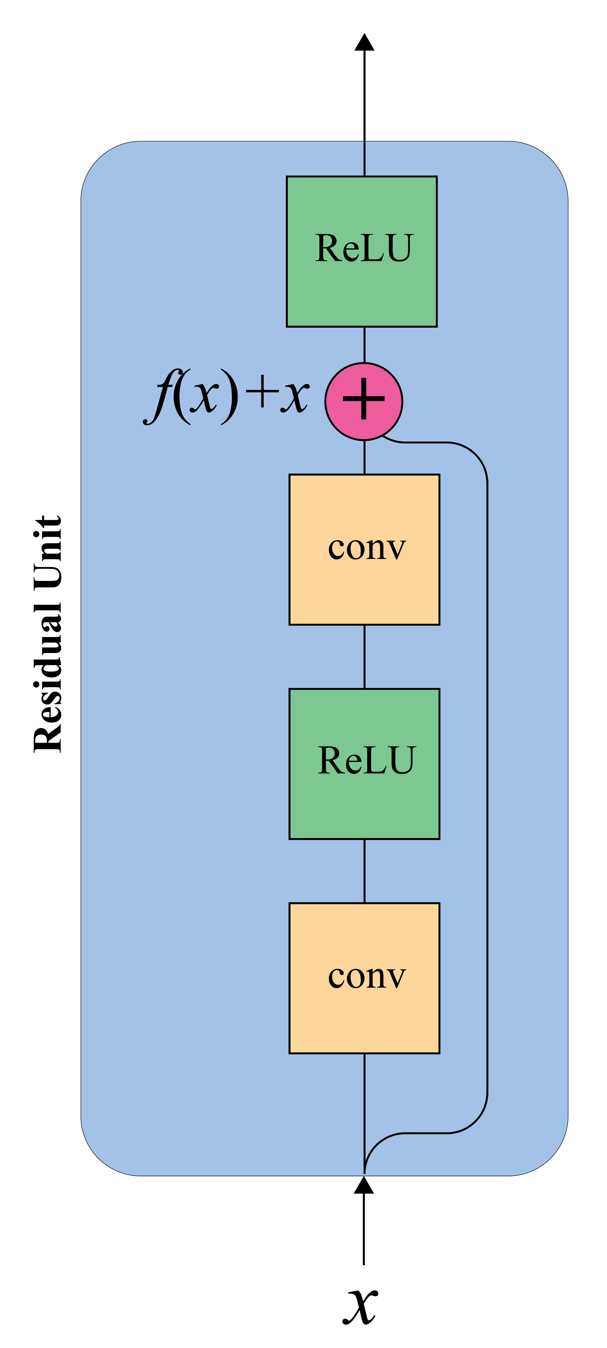
Residual unit
- Pass through connections adds the input of a layer to its output
- Deeper models are harder to train
- Learn residual function rather than direct mapping
- Notice the loss landscape with and without residual connections
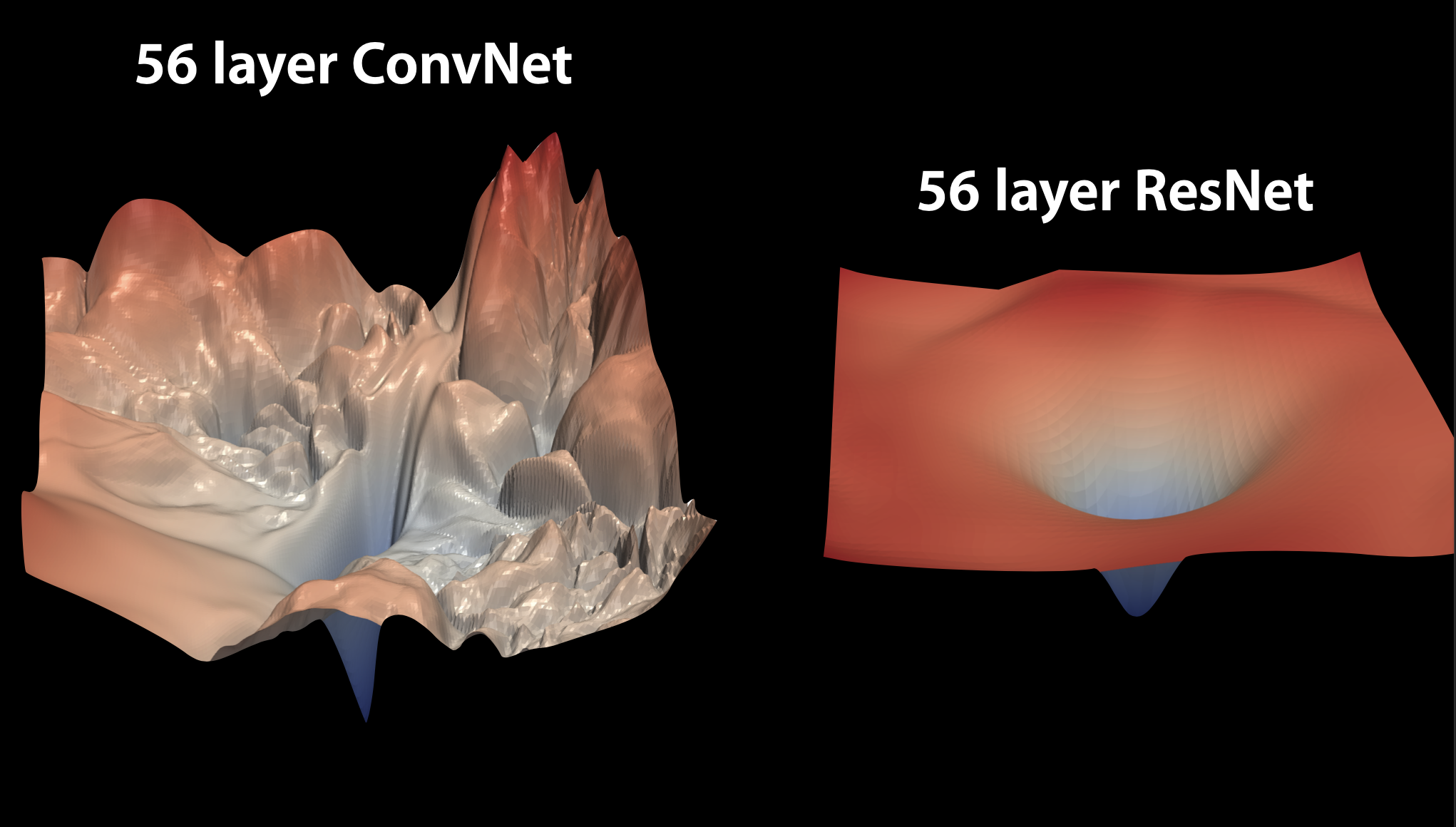
Figure taken from K. Derpanis notes on deep learning.
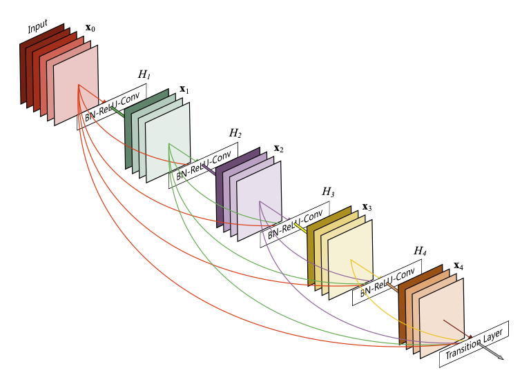
Figure from Huang et al. 2017.
- Feature-maps learned by any of the layers can be accessed by all subsequent layers.
- Encourages feature reuse throughout the network
- Leads to more compact models
- Supports diversified depth
- Improved training
- Individual layers get additional supervision from loss function through shorter (more direct) connections
- Similar to DSN (Lee et al. 2015) that attach classifiers to each hidden layer forcing intermediate layers to learn discriminative features
- Scale to hundreds of layers without any optimization difficulties
- Individual layers get additional supervision from loss function through shorter (more direct) connections
Dense blocks and transition layers
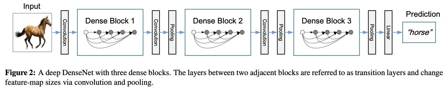
Figure from Huang et al. 2017
Densenet vs. Resnet
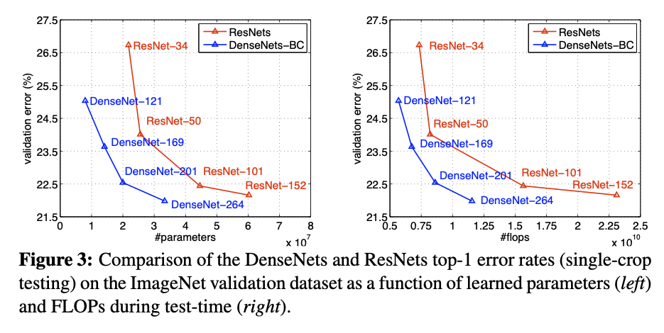
Figure from Huang et al. 2017
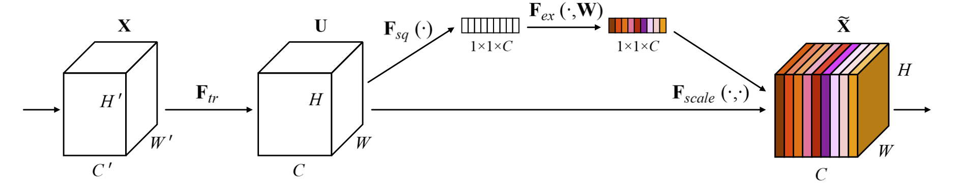
Figure from Hu et al. 2018
SE Block
- Squeeze operator
- Allows global information to be used when computing channel-wise weights
- Excitation operator
- Distribution across different classes is similar in early layers, suggesting that feature channels are "equally important" for different classes in early layers
- Distribution becomes class-specific in deeper layers
- SE blocks may be used for model prunning and network compression
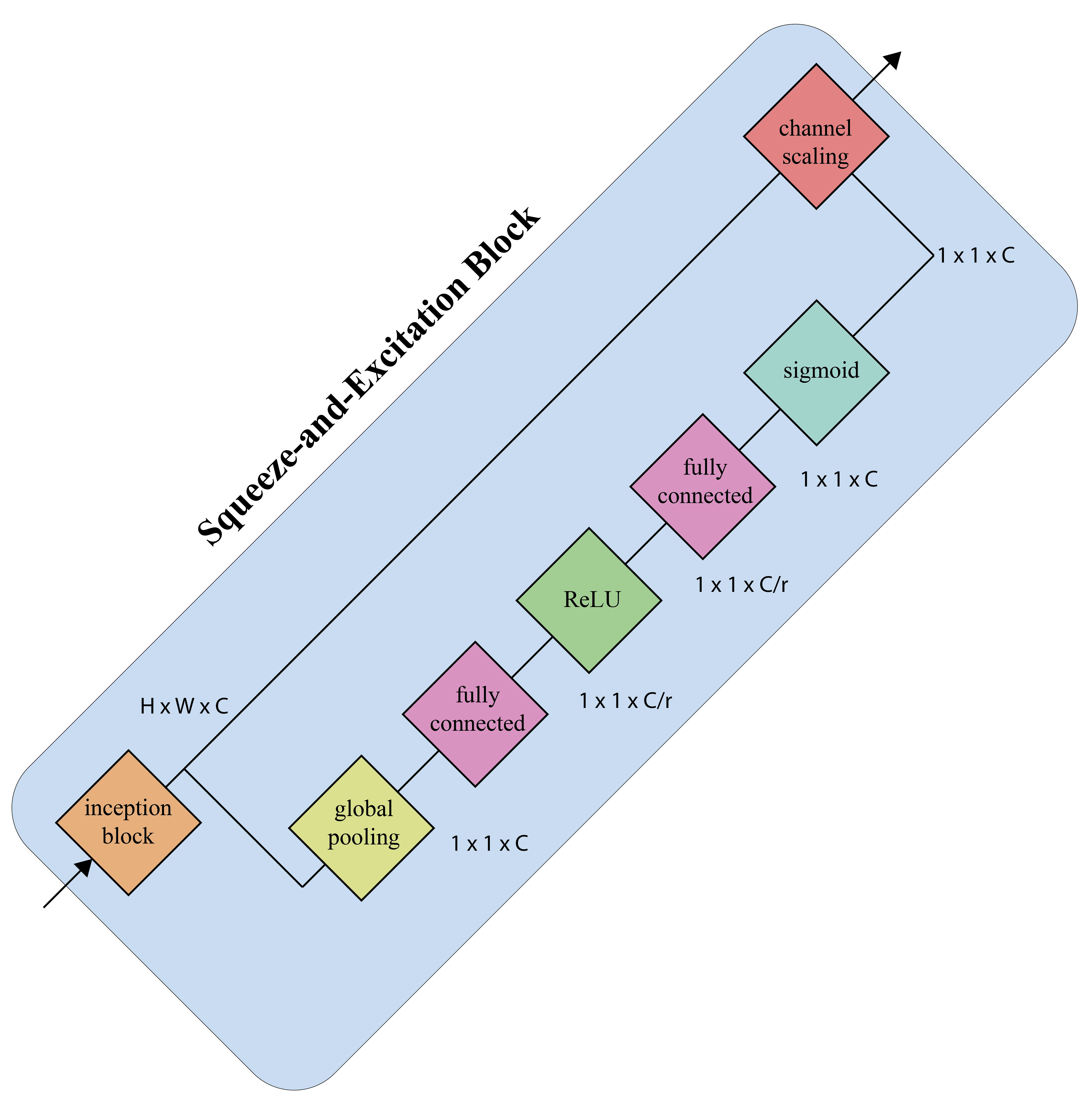
Squeeze-and-Excitation block (simplified).
SE Performance
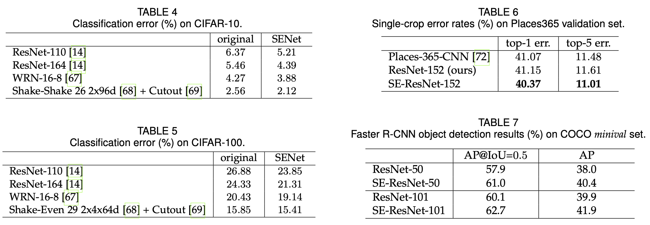
Taken from Hu et al. 2018
Spatial attention
- SE computes channel weights; however, we can easily extend this idea to compute spatial weights to model some notion of spatial attention
- The model will pay more attention to f
Other notable examples
FractalNet: Ultra-Deep Neural Networks without Residuals
SqueezeNet: AlexNet-Level Accuracy with 50x Fewer Parameters and <0.5MB Model Size
MobileNet: Efficient Convolutional Neural Networks for Mobile Vision Applications
Aggregated Residual Transformation for Deep Neural Networks
Deep Pyramidal Residual Networks
Xception: Deep Learning with Depthwise Separable Convolutions
Attention-based Networks
- Transformers use attention-based computation.
- These models are popular in Natural Language Processing community.
- GPT3 language model also uses attention-based computation and it has roughly 175 billion parameters.
Exploring Self-attention for Image Recognition
End-to-End Object Detection with Transformers
An Image is Worth 16x16 Words: Transformers for Image Recognition at Scale
Rethinking Semantic Segmentation from a Sequence-to-Sequence Perspective with Transformers
Learning convolution kernels
- Observation
- CNNs benefit from different kernel sizes at different layers
- Exploring all possible combinations of kernel sizes is infeasible in practice
FlexConv: Continuous Kernel Convolutions with Differentiable Kernel Sizes
Learning Strides in Convolutional Neural Networks
Do You Even Need Attention? A Stack of Feed-Forward Layers Does Surprising Well on ImageNet
ResMLP: Feedforward Networks for Image Classification with Data Efficient Training
- Results on ImageNet
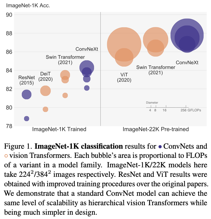
Figure from Lie et al. 2020
Modernizing a ConvNet towards Swin (Hierarchical Vision Transformer)
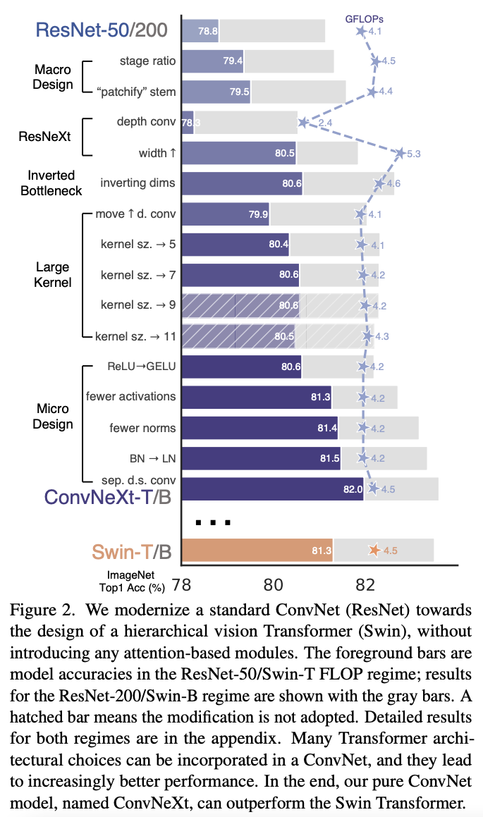
Figure from Lie et al. 2020
Key ideas
- Change stem to Patchify
Replace the ResNet-style stem cell with a patchify layer implemented using a $4 \times 4$, stride $4$ convolutional layer. The accuracy has changed from $79.4\%$ to $79.5\%$.
The stem cell in standard ResNet contains a $7 \times 7$ convolution layer with stride $2$, followed by a max pool, which results in a $4 \times$ downsampling of the input images.
- ResNeXtify
- Grouped convolutions idea from Xie et al. 2016
- Depthwise convolution where the number of groups equal to the number of channels. Similar to MobileNet and Xception.
- Only mixes information in the spatial domain.
- Depthwise convolution where the number of groups equal to the number of channels. Similar to MobileNet and Xception.
- Grouped convolutions idea from Xie et al. 2016
The combination of depthwise conv and $1 \times 1$ convs leads to a separation of spatial and channel mixing, a property shared by vision Transformers, where each operation either mixes information across spatial or channel dimension, but not both.
- Inverted bottleneck
One important design in every Transformer block is that it creates an inverted bottleneck, i.e., the hidden dimension of the MLP block is four times wider than the input dimension.
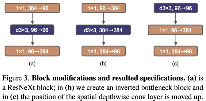
Figure from Lie et al. 2020
- Large kernel sizes
One of the most distinguishing aspects of vision Transformers is their non-local self-attention, which enables each layer to have a global receptive field.
To explore large kernels, one prerequisite is to move up the position of the depthwise conv layer.
- Replacing ReLU with GELU
- Gaussian Error Linear Unit (Hendrycks and Gimpel, 2016)
- Use fewer activation functions
- Use fewer normalization layers
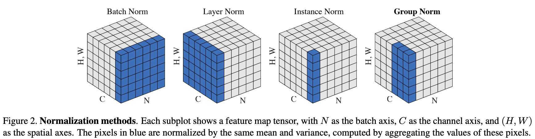
- Replace batch normalization with layer normalization
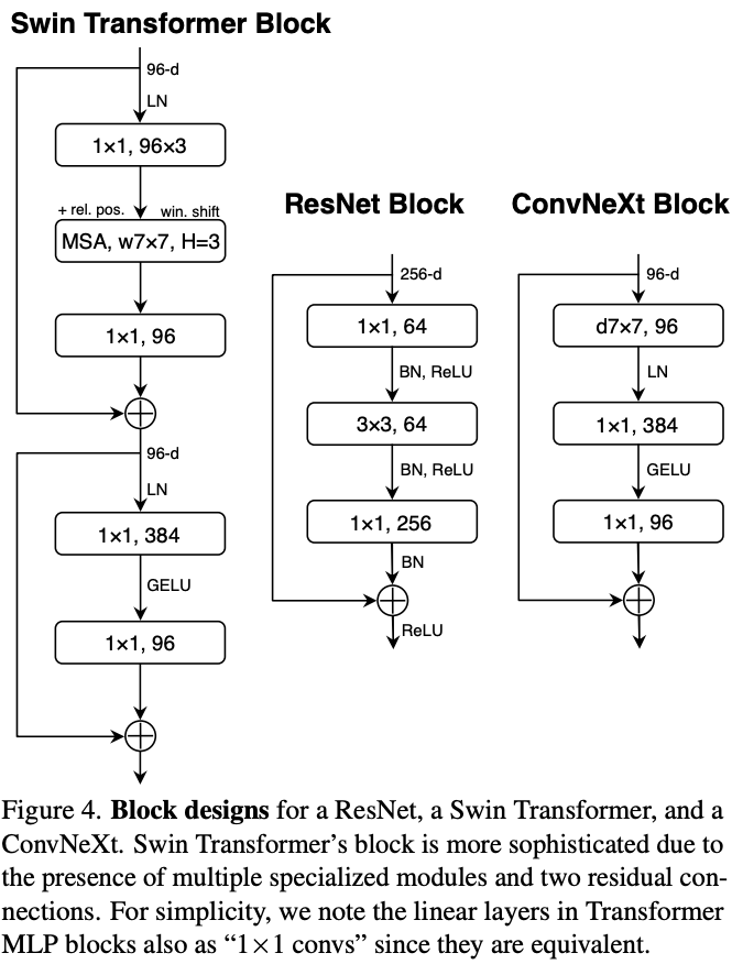
Figure from Lie et al. 2020
Is object detection solved?
ObjectNet: A Large-Scale Bias-Controlled Dataset for Pushing the Limits of Object Recognition Models`
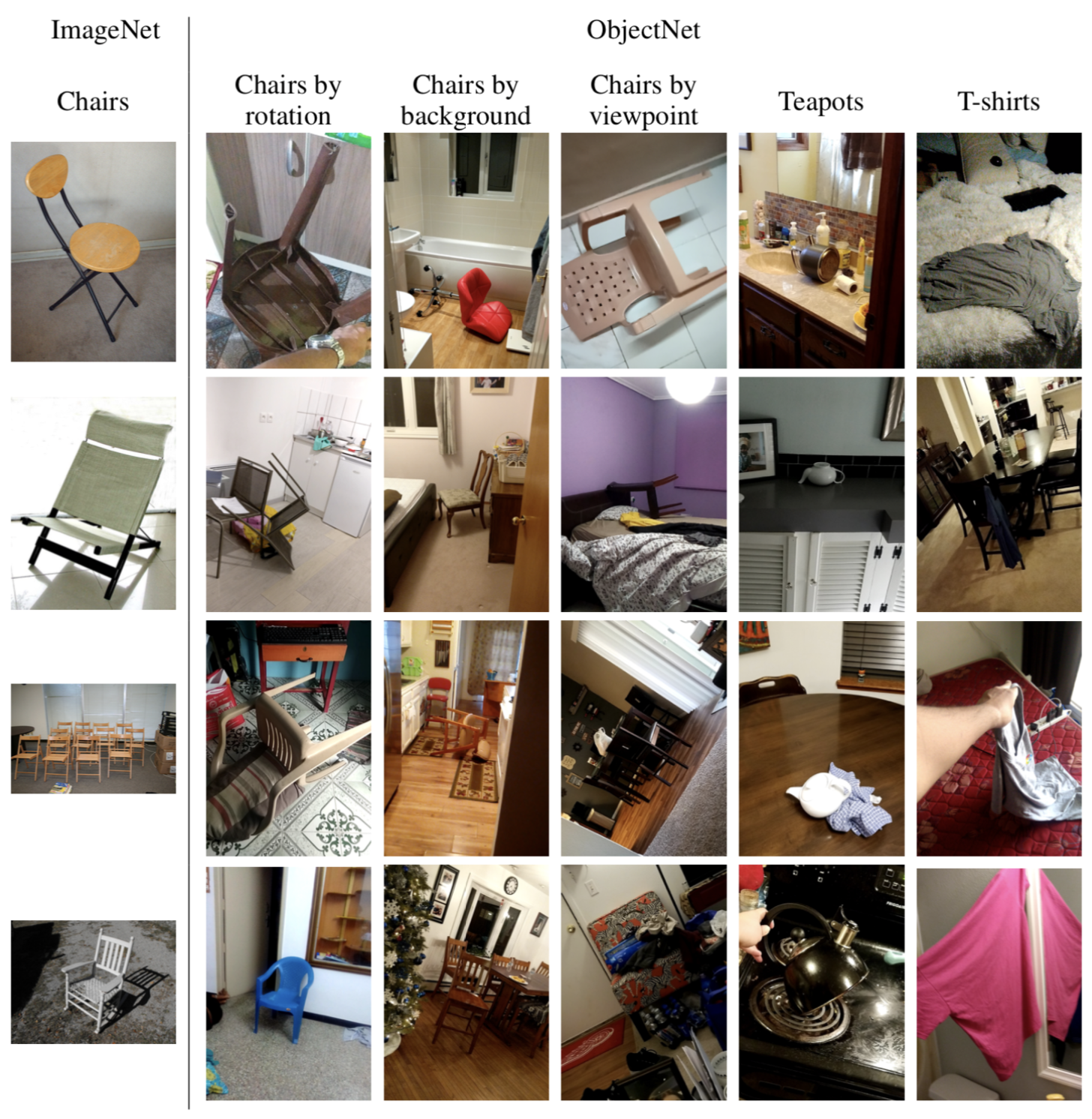
Figure taken from objectnet.dev
- Performance on ObjectNet benchmark
- 40 to 45% drop in performance
Afterward
- Adapted from Jeff Hawkins, Founder of Palm Computing.
The key to object recognition is representation.
- Convolutional neural networks are particularly well-suited for computer vision tasks
- Convolutional layers "mimic" processing in visual cortex
- Exploits spatial relationship between neighbouring pixels
- Learns powerful representations that reduce the semantic gap
Practical matters: where to go from here?
- Deep learning is as much about engineering as it is about science
- Learn one of deep learning frameworks
- Become an efficient coder
- Don't be afraid to use high-level deep learning tools to quickly prototype baselines (e.g., huggingface)
- Deep learning projects share common features
- Data loaders
- Measuring performance, say accuracy, precision, etc.
- Deep learning projects share common features